Demo: RAIL Evaluation

Authors: Sam Schmidt, Alex Malz, Julia Gschwend, others…

Last run successfully: June 16, 2023 (with qp-prob >= 0.8.2)

The purpose of this notebook is to demonstrate the application of the metrics scripts to be used on the photo-z PDF catalogs produced by the PZ working group. The first implementation of the evaluation module is based on the refactoring of the code used in Schmidt et al. 2020, available on Github repository PZDC1paper.

To run this notebook, you must install qp and have the notebook in the same directory as utils.py (available in RAIL’s examples directrory). You must also have installed all RAIL dependencies, particularly for the estimation codes that you want to run, as well as ceci, qp, tables_io, etc… See the RAIL installation instructions for more info.

Note: If you’re planning to run this in a notebook, you may want to use interactive mode instead. See Single_Evaluation.ipynb in the interactive_examples/evaluation_examples/ folder for a version of this notebook in interactive mode.

import rail
from rail.evaluation.metrics.cdeloss import *
from rail.evaluation.evaluator import OldEvaluator
from rail.core.data import QPHandle, TableHandle, Hdf5Handle
from rail.core.stage import RailStage
from utils import plot_pit_qq, ks_plot
import qp
import tables_io
import os
%matplotlib inline
%reload_ext autoreload
%autoreload 2

Data

To compute the photo-z metrics of a given test sample, it is necessary to read the output of a photo-z code containing galaxies’ photo-z PDFs. Let’s use the toy data available in tests/data/ (test_dc2_training_9816.hdf5 and test_dc2_validation_9816.hdf5) to generate a small sample of photo-z PDFs using the FlexZBoost algorithm available on RAIL’s estimation module.

Photo-z Results

Run FlexZBoost

If you have run the notebook RAIL_estimation_demo.ipynb, this will produce a file output_fzboost.hdf5, writen at the location: <your_path>/RAIL/examples/estimation_examples/output_fzboost.hdf5.

Otherwise we can download the file from NERSC

Next we need to set up some paths for the Data Store:

from rail.utils.path_utils import find_rail_file
try:
    pdfs_file = find_rail_file('examples_data/evaluation_data/data/output_fzboost.hdf5')
except ValueError:
    pdfs_file = 'examples_data/evaluation_data/data/output_fzboost.hdf5'
    try:
        os.makedirs(os.path.dirname(pdfs_file))
    except FileExistsError:
        pass
    curl_com = f"curl -o {pdfs_file} https://portal.nersc.gov/cfs/lsst/PZ/output_fzboost.hdf5"
    os.system(curl_com)
ztrue_file = find_rail_file('examples_data/testdata/test_dc2_validation_9816.hdf5')

    % Total    % Received % Xferd  Average Speed   Time    Time     Time  Current
                                   Dload  Upload   Total   Spent    Left  Speed

0     0    0     0    0     0      0      0 --:--:-- --:--:-- --:--:--     0
0     0    0     0    0     0      0      0 --:--:-- --:--:-- --:--:--     0

53 47.1M   53 25.0M    0     0  23.0M      0  0:00:02  0:00:01  0:00:01 23.0M

100 47.1M 100 47.1M 0 0 33.2M 0 0:00:01 0:00:01 –:–:– 33.2M

Read the data in, note that the fzdata is a qp Ensemble, and thus we should read it in as a QPHandle type file, while the ztrue_data is tabular data, and should be read in as a Tablehandle when adding to the data store

fzdata = qp.read(pdfs_file)
ztrue_data = tables_io.read(ztrue_file)

ztrue = ztrue_data['photometry']['redshift']
zgrid = fzdata.metadata['xvals'].ravel()
photoz_mode = fzdata.mode(grid=zgrid)

truth = Hdf5Handle('truth', data=ztrue_data['photometry'])
ensemble = QPHandle('ensemble',data=fzdata)

Make an evaulator stage

Now let’s set up the Evaluator stage to compute our metrics for the FlexZBoost results

FZB_eval = OldEvaluator.make_stage(name='FZB_eval', truth=truth, output_mode="return")

FZB_results = FZB_eval.evaluate(ensemble(), truth)

Inserting handle into data store.  input: None, FZB_eval
Inserting handle into data store.  truth: <class 'rail.core.data.Hdf5Handle'> None, (d), FZB_eval

/opt/hostedtoolcache/Python/3.10.20/x64/lib/python3.10/site-packages/qp/metrics/array_metrics.py:27: UserWarning: p-value floored: true value smaller than 0.001. Consider specifying method (e.g. method=stats.PermutationMethod().)
  return stats.anderson_ksamp([p_random_variables, q_random_variables], **kwargs)

Inserting handle into data store.  output_FZB_eval: inprogress_output_FZB_eval.hdf5, FZB_eval

We can view the results as a pandas dataframe:

results_df= tables_io.convertObj(FZB_results(), tables_io.types.PD_DATAFRAME)
results_df

	PIT_AD_stat	PIT_AD_pval	PIT_AD_significance_level	PIT_CvM_stat	PIT_CvM_pval	PIT_KS_stat	PIT_KS_pval	PIT_OutRate_stat	POINT_SimgaIQR	POINT_Bias	POINT_OutlierRate	POINT_SigmaMAD	CDE_stat
0	84.956236	NaN	0.001	9.623352	NaN	0.03359	NaN	0.058738	0.020859	0.00027	0.106167	0.020891	-6.74027

So, there we have it, a way to generate all of our summary statistics for FZBoost. And note also that the results file has been written out to output_FZB_eval.hdf5, the name we specified when we ran make_stage (with output_ prepended).

As an alternative, and to allow for a little more explanation for each individual metric, we can calculate the metrics using functions from the evaluation class separate from the stage infrastructure. Here are some examples below.

CDF-based Metrics

PIT

The Probability Integral Transform (PIT), is the Cumulative Distribution Function (CDF) of the photo-z PDF

\[\mathrm{CDF}(f, q)\ =\ \int_{-\infty}^{q}\ f(z)\ dz\]

evaluated at the galaxy’s true redshift for every galaxy \(i\) in the catalog.

\[\mathrm{PIT}(p_{i}(z);\ z_{i})\ =\ \int_{-\infty}^{z^{true}_{i}}\ p_{i}(z)\ dz\]

from qp.metrics.pit import PIT
pitobj = PIT(fzdata, ztrue)
quant_ens = pitobj.pit
metamets = pitobj.calculate_pit_meta_metrics()

/opt/hostedtoolcache/Python/3.10.20/x64/lib/python3.10/site-packages/qp/metrics/array_metrics.py:27: UserWarning: p-value floored: true value smaller than 0.001. Consider specifying method (e.g. method=stats.PermutationMethod().)
  return stats.anderson_ksamp([p_random_variables, q_random_variables], **kwargs)

The evaluate method PIT class returns two objects, a quantile distribution based on the full set of PIT values (a frozen distribution object), and a dictionary of meta metrics associated to PIT (to be detailed below).

quant_ens

Ensemble(the_class=quant,shape=(1, 96))

metamets

{'ad': Anderson_ksampResult(statistic=np.float64(84.95623553609381), critical_values=array([0.325, 1.226, 1.961, 2.718, 3.752, 4.592, 6.546]), pvalue=np.float64(0.001)),
 'cvm': CramerVonMisesResult(statistic=9.62335199605935, pvalue=9.265039846440004e-10),
 'ks': KstestResult(statistic=np.float64(0.033590049370962216), pvalue=np.float64(1.7621068075751534e-20), statistic_location=np.float64(0.9921210288809627), statistic_sign=np.int8(-1)),
 'outlier_rate': np.float64(0.05873797877466336)}

PIT values

pit_vals = np.array(pitobj.pit_samps)
pit_vals

array([0.19392947, 0.36675619, 0.52017547, ..., 1.        , 0.93189232,
       0.4674437 ], shape=(20449,))

PIT outlier rate

The PIT outlier rate is a global metric defined as the fraction of galaxies in the sample with extreme PIT values. The lower and upper limits for considering a PIT as outlier are optional parameters set at the Metrics instantiation (default values are: PIT \(<10^{-4}\) or PIT \(>0.9999\)).

pit_out_rate = metamets['outlier_rate']
print(f"PIT outlier rate of this sample: {pit_out_rate:.6f}")
pit_out_rate = pitobj.evaluate_PIT_outlier_rate()
print(f"PIT outlier rate of this sample: {pit_out_rate:.6f}")

PIT outlier rate of this sample: 0.058738
PIT outlier rate of this sample: 0.058738

PIT-QQ plot

The histogram of PIT values is a useful tool for a qualitative assessment of PDFs quality. It shows whether the PDFs are: * biased (tilted PIT histogram) * under-dispersed (excess counts close to the boudaries 0 and 1) * over-dispersed (lack of counts close the boudaries 0 and 1) * well-calibrated (flat histogram)

Following the standards in DC1 paper, the PIT histogram is accompanied by the quantile-quantile (QQ), which can be used to compare qualitatively the PIT distribution obtained with the PDFs agaist the ideal case (uniform distribution). The closer the QQ plot is to the diagonal, the better is the PDFs calibration.

pdfs = fzdata.objdata['yvals']
plot_pit_qq(pdfs, zgrid, ztrue, title="PIT-QQ - toy data", code="FlexZBoost",
                pit_out_rate=pit_out_rate, savefig=False)

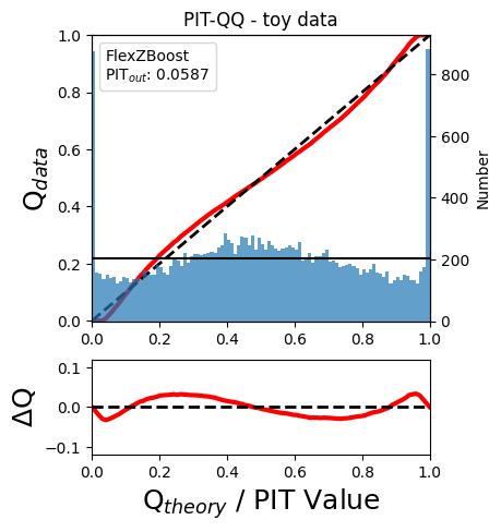
../../../_images/00_Single_Evaluation_30_0.png

The black horizontal line represents the ideal case where the PIT histogram would behave as a uniform distribution U(0,1).

Summary statistics of CDF-based metrics

To evaluate globally the quality of PDFs estimates, rail.evaluation provides a set of metrics to compare the empirical distributions of PIT values with the reference uniform distribution, U(0,1).

Kolmogorov-Smirnov

Let’s start with the traditional Kolmogorov-Smirnov (KS) statistic test, which is the maximum difference between the empirical and the expected cumulative distributions of PIT values:

\[\mathrm{KS} \equiv \max_{PIT} \Big( \left| \ \mathrm{CDF} \small[ \hat{f}, z \small] - \mathrm{CDF} \small[ \tilde{f}, z \small] \ \right| \Big)\]

Where \(\hat{f}\) is the PIT distribution and \(\tilde{f}\) is U(0,1). Therefore, the smaller value of KS the closer the PIT distribution is to be uniform. The evaluate method of the PITKS class returns a named tuple with the statistic and p-value.

ks_stat_and_pval = metamets['ks']
print(f"PIT KS stat and pval: {ks_stat_and_pval}")
ks_stat_and_pval = pitobj.evaluate_PIT_KS()
print(f"PIT KS stat and pval: {ks_stat_and_pval}")

PIT KS stat and pval: KstestResult(statistic=np.float64(0.033590049370962216), pvalue=np.float64(1.7621068075751534e-20), statistic_location=np.float64(0.9921210288809627), statistic_sign=np.int8(-1))
PIT KS stat and pval: KstestResult(statistic=np.float64(0.033590049370962216), pvalue=np.float64(1.7621068075751534e-20), statistic_location=np.float64(0.9921210288809627), statistic_sign=np.int8(-1))

Visual interpretation of the KS statistic:

ks_plot(pitobj)

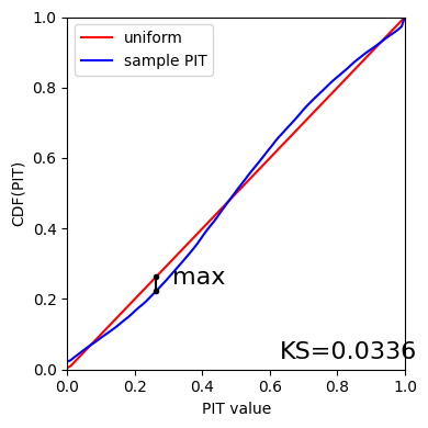
../../../_images/00_Single_Evaluation_36_0.png

print(f"KS metric of this sample: {ks_stat_and_pval.statistic:.4f}")

KS metric of this sample: 0.0336

Cramer-von Mises

Similarly, let’s calculate the Cramer-von Mises (CvM) test, a variant of the KS statistic defined as the mean-square difference between the CDFs of an empirical PDF and the true PDFs:

\[\mathrm{CvM}^2 \equiv \int_{-\infty}^{\infty} \Big( \mathrm{CDF} \small[ \hat{f}, z \small] \ - \ \mathrm{CDF} \small[ \tilde{f}, z \small] \Big)^{2} \mathrm{dCDF}(\tilde{f}, z)\]

on the distribution of PIT values, which should be uniform if the PDFs are perfect.

cvm_stat_and_pval = metamets['cvm']
print(f"PIT CvM stat and pval: {cvm_stat_and_pval}")
cvm_stat_and_pval = pitobj.evaluate_PIT_CvM()
print(f"PIT CvM stat and pval: {cvm_stat_and_pval}")

PIT CvM stat and pval: CramerVonMisesResult(statistic=9.62335199605935, pvalue=9.265039846440004e-10)
PIT CvM stat and pval: CramerVonMisesResult(statistic=9.62335199605935, pvalue=9.265039846440004e-10)

print(f"CvM metric of this sample: {cvm_stat_and_pval.statistic:.4f}")

CvM metric of this sample: 9.6234

Anderson-Darling

Another variation of the KS statistic is the Anderson-Darling (AD) test, a weighted mean-squared difference featuring enhanced sensitivity to discrepancies in the tails of the distribution.

\[\mathrm{AD}^2 \equiv N_{tot} \int_{-\infty}^{\infty} \frac{\big( \mathrm{CDF} \small[ \hat{f}, z \small] \ - \ \mathrm{CDF} \small[ \tilde{f}, z \small] \big)^{2}}{\mathrm{CDF} \small[ \tilde{f}, z \small] \big( 1 \ - \ \mathrm{CDF} \small[ \tilde{f}, z \small] \big)}\mathrm{dCDF}(\tilde{f}, z)\]

ad_stat_crit_sig = metamets['ad']
print(f"PIT AD stat and pval: {ad_stat_crit_sig}")
ad_stat_crit_sig = pitobj.evaluate_PIT_anderson_ksamp()
print(f"PIT AD stat and pval: {ad_stat_crit_sig}")

PIT AD stat and pval: Anderson_ksampResult(statistic=np.float64(84.95623553609381), critical_values=array([0.325, 1.226, 1.961, 2.718, 3.752, 4.592, 6.546]), pvalue=np.float64(0.001))
PIT AD stat and pval: Anderson_ksampResult(statistic=np.float64(84.95623553609381), critical_values=array([0.325, 1.226, 1.961, 2.718, 3.752, 4.592, 6.546]), pvalue=np.float64(0.001))

print(f"AD metric of this sample: {ad_stat_crit_sig.statistic:.4f}")

AD metric of this sample: 84.9562

It is possible to remove catastrophic outliers before calculating the integral for the sake of preserving numerical instability. For instance, Schmidt et al. computed the Anderson-Darling statistic within the interval (0.01, 0.99).

ad_stat_crit_sig_cut = pitobj.evaluate_PIT_anderson_ksamp(pit_min=0.01, pit_max=0.99)
print(f"AD metric of this sample: {ad_stat_crit_sig.statistic:.4f}")
print(f"AD metric for 0.01 < PIT < 0.99: {ad_stat_crit_sig_cut.statistic:.4f}")

WARNING:root:Removed 1760 PITs from the sample.

AD metric of this sample: 84.9562
AD metric for 0.01 < PIT < 0.99: 89.9826

CDE Loss

In the absence of true photo-z posteriors, the metric used to evaluate individual PDFs is the Conditional Density Estimate (CDE) Loss, a metric analogue to the root-mean-squared-error:

\[L(f, \hat{f}) \equiv \int \int {\big(f(z | x) - \hat{f}(z | x) \big)}^{2} dzdP(x),\]

where \(f(z | x)\) is the true photo-z PDF and \(\hat{f}(z | x)\) is the estimated PDF in terms of the photometry \(x\). Since \(f(z | x)\) is unknown, we estimate the CDE Loss as described in Izbicki & Lee, 2017 (arXiv:1704.08095). :

\[\mathrm{CDE} = \mathbb{E}\big( \int{{\hat{f}(z | X)}^2 dz} \big) - 2{\mathbb{E}}_{X, Z}\big(\hat{f}(Z, X) \big) + K_{f},\]

where the first term is the expectation value of photo-z posterior with respect to the marginal distribution of the covariates X, and the second term is the expectation value with respect to the joint distribution of observables X and the space Z of all possible redshifts (in practice, the centroids of the PDF bins), and the third term is a constant depending on the true conditional densities \(f(z | x)\).

cdelossobj = CDELoss(fzdata, zgrid, ztrue)

cde_stat_and_pval = cdelossobj.evaluate()
cde_stat_and_pval

stat_and_pval(statistic=np.float64(-6.725602928688286), p_value=nan)

print(f"CDE loss of this sample: {cde_stat_and_pval.statistic:.2f}")

CDE loss of this sample: -6.73

We note that all of the quantities as run individually are identical to the quantities in our summary table - a nice check that things have run properly.