RAIL’s DNF implementation example
Authors: Laura Toribio San Cipriano, Sam Schmidt and Juan De Vicente last successfully run: Feb 9, 2026
This is a notebook demonstrating some of the features of the LSSTDESC
RAIL version of the DNF estimator, see De Vicente et
al. (2016) for more details on the
algorithm.
Note: If you’re interested in running this in pipeline mode, see
05_DNF.ipynb
in the pipeline_examples/estimation_examples/ folder.
DNF (Directional Neighbourhood Fitting) is a nearest-neighbor approach for photometric redshift estimation developed at the CIEMAT (Centro de Investigaciones Energéticas, Medioambientales y Tecnológicas) at Madrid. DNF computes the photo-z hyperplane that best fits the directional neighbourhood of a photometric galaxy in the training sample.
The current version of the code for RAILconsists of a training
stage, DNFInformer and a estimation stage DNFEstimator.
DNFInformer is a class that preprocesses the protometric data,
handles missing or non-detected values, and trains a first basic
k-Nearest Neighbors regressor for redshift prediction. The
DNFEstimator calculates photometric redshifts based on an
enhancement of Nearest Neighbor techniques. The class supports three
main metrics for redshift estimation: ENF, ANF or DNF.
ENF: Euclidean neighbourhood. It’s a common distance metric used in kNN (k-Nearest Neighbors) for photometric redshift prediction.
ANF: uses normalized inner product for more accurate photo-z predictions. It is particularly recommended when working with datasets containing more than four filters.
DNF: combines Euclidean and angular metrics, improving accuracy, especially for larger neighborhoods, and maintaining proportionality in observable content.
DNFInformer
The DNFInformer class processes a training dataset and produces a
model file containing the computed magnitudes, colors, and their
associated errors for the dataset. This model is then utilized in the
DNFEstimator stage for photometric redshift estimation. Missing
photometric detections (non-detections) are handled by replacing them
with a configurable placeholder value, or optionally ignoring them
during model training.
The configurable parameters for DNFInformer include:
bands: List of band names expected in the input dataset.err_bands: List of magnitude error column names corresponding to the bands.redshift_col: String indicating the name of the redshift column in the input data.mag_limits: Dictionary with band names as keys and floats representing the acceptable magnitude range for each band.nondetect_val: Float or np.nan, the value indicating a non-detection, which will be replaced by the values in mag_limits.replace_nondetect: Boolean; if True, non-detections are replaced with the specified nondetect_val. If False, non-detections are ignored during the neighbor-finding process.
DNFEstimator
The DNFEstimator class uses the model generated by DNFInformer to
compute photometric redshifts for new datasets and the PDFs. It
identifies the nearest neighbors from the training data using various
distance metrics and estimates redshifts based on these neighbors.
The configurable parameters for DNFEstimator include:
bands,err_bands,redshift_col,nondetect_val,mag_limits: As described forDNFInformer.selection_mode: Integer indicating the method for neighbor selection:0: Euclidean Neighbourhood Fitting (ENF).1: Angular Neighbourhood Fitting (ANF).2: Directional Neighbourhood Fitting (DNF).
zmin,zmax,nzbins: Float values defining the minimum and maximum redshift range and the number of bins for estimation of the PDFs.pdf_estimation: Boolean; if True, computes a probability density function (PDF) for the redshift of each object.
import matplotlib.pyplot as plt
import numpy as np
import tables_io
from rail.utils.path_utils import find_rail_file

from rail import interactive as ri
Install FSPS with the following commands:
pip uninstall fsps
git clone --recursive https://github.com/dfm/python-fsps.git
cd python-fsps
python -m pip install .
export SPS_HOME=$(pwd)/src/fsps/libfsps

LEPHAREDIR is being set to the default cache directory:
/home/runner/.cache/lephare/data
More than 1Gb may be written there.
LEPHAREWORK is being set to the default cache directory:
/home/runner/.cache/lephare/work
Default work cache is already linked.
This is linked to the run directory:
/home/runner/.cache/lephare/runs/20260504T123336
A module that was compiled using NumPy 1.x cannot be run in
NumPy 2.2.6 as it may crash. To support both 1.x and 2.x
versions of NumPy, modules must be compiled with NumPy 2.0.
Some module may need to rebuild instead e.g. with 'pybind11>=2.12'.

If you are a user of the module, the easiest solution will be to
downgrade to 'numpy<2' or try to upgrade the affected module.
We expect that some modules will need time to support NumPy 2.

Traceback (most recent call last):  File "/opt/hostedtoolcache/Python/3.10.20/x64/lib/python3.10/runpy.py", line 196, in _run_module_as_main
    return _run_code(code, main_globals, None,
  File "/opt/hostedtoolcache/Python/3.10.20/x64/lib/python3.10/runpy.py", line 86, in _run_code
    exec(code, run_globals)
  File "/opt/hostedtoolcache/Python/3.10.20/x64/lib/python3.10/site-packages/ipykernel_launcher.py", line 18, in <module>
    app.launch_new_instance()
  File "/opt/hostedtoolcache/Python/3.10.20/x64/lib/python3.10/site-packages/traitlets/config/application.py", line 1075, in launch_instance
    app.start()
  File "/opt/hostedtoolcache/Python/3.10.20/x64/lib/python3.10/site-packages/ipykernel/kernelapp.py", line 758, in start
    self.io_loop.start()
  File "/opt/hostedtoolcache/Python/3.10.20/x64/lib/python3.10/site-packages/tornado/platform/asyncio.py", line 211, in start
    self.asyncio_loop.run_forever()
  File "/opt/hostedtoolcache/Python/3.10.20/x64/lib/python3.10/asyncio/base_events.py", line 603, in run_forever
    self._run_once()
  File "/opt/hostedtoolcache/Python/3.10.20/x64/lib/python3.10/asyncio/base_events.py", line 1909, in _run_once
    handle._run()
  File "/opt/hostedtoolcache/Python/3.10.20/x64/lib/python3.10/asyncio/events.py", line 80, in _run
    self._context.run(self._callback, *self._args)
  File "/opt/hostedtoolcache/Python/3.10.20/x64/lib/python3.10/site-packages/ipykernel/utils.py", line 71, in preserve_context
    return await f(*args, **kwargs)
  File "/opt/hostedtoolcache/Python/3.10.20/x64/lib/python3.10/site-packages/ipykernel/kernelbase.py", line 621, in shell_main
    await self.dispatch_shell(msg, subshell_id=subshell_id)
  File "/opt/hostedtoolcache/Python/3.10.20/x64/lib/python3.10/site-packages/ipykernel/kernelbase.py", line 478, in dispatch_shell
    await result
  File "/opt/hostedtoolcache/Python/3.10.20/x64/lib/python3.10/site-packages/ipykernel/ipkernel.py", line 372, in execute_request
    await super().execute_request(stream, ident, parent)
  File "/opt/hostedtoolcache/Python/3.10.20/x64/lib/python3.10/site-packages/ipykernel/kernelbase.py", line 834, in execute_request
    reply_content = await reply_content
  File "/opt/hostedtoolcache/Python/3.10.20/x64/lib/python3.10/site-packages/ipykernel/ipkernel.py", line 464, in do_execute
    res = shell.run_cell(
  File "/opt/hostedtoolcache/Python/3.10.20/x64/lib/python3.10/site-packages/ipykernel/zmqshell.py", line 663, in run_cell
    return super().run_cell(*args, **kwargs)
  File "/opt/hostedtoolcache/Python/3.10.20/x64/lib/python3.10/site-packages/IPython/core/interactiveshell.py", line 3077, in run_cell
    result = self._run_cell(
  File "/opt/hostedtoolcache/Python/3.10.20/x64/lib/python3.10/site-packages/IPython/core/interactiveshell.py", line 3132, in _run_cell
    result = runner(coro)
  File "/opt/hostedtoolcache/Python/3.10.20/x64/lib/python3.10/site-packages/IPython/core/async_helpers.py", line 128, in _pseudo_sync_runner
    coro.send(None)
  File "/opt/hostedtoolcache/Python/3.10.20/x64/lib/python3.10/site-packages/IPython/core/interactiveshell.py", line 3336, in run_cell_async
    has_raised = await self.run_ast_nodes(code_ast.body, cell_name,
  File "/opt/hostedtoolcache/Python/3.10.20/x64/lib/python3.10/site-packages/IPython/core/interactiveshell.py", line 3519, in run_ast_nodes
    if await self.run_code(code, result, async_=asy):
  File "/opt/hostedtoolcache/Python/3.10.20/x64/lib/python3.10/site-packages/IPython/core/interactiveshell.py", line 3579, in run_code
    exec(code_obj, self.user_global_ns, self.user_ns)
  File "/tmp/ipykernel_5205/444981919.py", line 6, in <module>
    from rail import interactive as ri
  File "/opt/hostedtoolcache/Python/3.10.20/x64/lib/python3.10/site-packages/rail/interactive/__init__.py", line 3, in <module>
    from . import calib, creation, estimation, evaluation, tools
  File "/opt/hostedtoolcache/Python/3.10.20/x64/lib/python3.10/site-packages/rail/interactive/calib/__init__.py", line 3, in <module>
    from rail.utils.interactive.initialize_utils import _initialize_interactive_module
  File "/opt/hostedtoolcache/Python/3.10.20/x64/lib/python3.10/site-packages/rail/utils/interactive/initialize_utils.py", line 17, in <module>
    from rail.utils.interactive.base_utils import (
  File "/opt/hostedtoolcache/Python/3.10.20/x64/lib/python3.10/site-packages/rail/utils/interactive/base_utils.py", line 10, in <module>
    rail.stages.import_and_attach_all(silent=True)
  File "/opt/hostedtoolcache/Python/3.10.20/x64/lib/python3.10/site-packages/rail/stages/__init__.py", line 74, in import_and_attach_all
    RailEnv.import_all_packages(silent=silent)
  File "/opt/hostedtoolcache/Python/3.10.20/x64/lib/python3.10/site-packages/rail/core/introspection.py", line 541, in import_all_packages
    _imported_module = importlib.import_module(pkg)
  File "/opt/hostedtoolcache/Python/3.10.20/x64/lib/python3.10/importlib/__init__.py", line 126, in import_module
    return _bootstrap._gcd_import(name[level:], package, level)
  File "/opt/hostedtoolcache/Python/3.10.20/x64/lib/python3.10/site-packages/rail/som/__init__.py", line 1, in <module>
    from rail.creation.degraders.specz_som import *
  File "/opt/hostedtoolcache/Python/3.10.20/x64/lib/python3.10/site-packages/rail/creation/degraders/specz_som.py", line 15, in <module>
    from somoclu import Somoclu
  File "/opt/hostedtoolcache/Python/3.10.20/x64/lib/python3.10/site-packages/somoclu/__init__.py", line 11, in <module>
    from .train import Somoclu
  File "/opt/hostedtoolcache/Python/3.10.20/x64/lib/python3.10/site-packages/somoclu/train.py", line 25, in <module>
    from .somoclu_wrap import train as wrap_train
  File "/opt/hostedtoolcache/Python/3.10.20/x64/lib/python3.10/site-packages/somoclu/somoclu_wrap.py", line 11, in <module>
    import _somoclu_wrap
---------------------------------------------------------------------------

ImportError                               Traceback (most recent call last)

File /opt/hostedtoolcache/Python/3.10.20/x64/lib/python3.10/site-packages/numpy/core/_multiarray_umath.py:44, in __getattr__(attr_name)
     39     # Also print the message (with traceback).  This is because old versions
     40     # of NumPy unfortunately set up the import to replace (and hide) the
     41     # error.  The traceback shouldn't be needed, but e.g. pytest plugins
     42     # seem to swallow it and we should be failing anyway...
     43     sys.stderr.write(msg + tb_msg)
---> 44     raise ImportError(msg)
     46 ret = getattr(_multiarray_umath, attr_name, None)
     47 if ret is None:


ImportError:
A module that was compiled using NumPy 1.x cannot be run in
NumPy 2.2.6 as it may crash. To support both 1.x and 2.x
versions of NumPy, modules must be compiled with NumPy 2.0.
Some module may need to rebuild instead e.g. with 'pybind11>=2.12'.

If you are a user of the module, the easiest solution will be to
downgrade to 'numpy<2' or try to upgrade the affected module.
We expect that some modules will need time to support NumPy 2.
Warning: the binary library cannot be imported. You cannot train maps, but you can load and analyze ones that you have already saved.
The problem occurs because either compilation failed when you installed Somoclu or a path is missing from the dependencies when you are trying to import it. Please refer to the documentation to see your options.
trainFile = find_rail_file("examples_data/testdata/test_dc2_training_9816.hdf5")
testFile = find_rail_file("examples_data/testdata/test_dc2_validation_9816.hdf5")
training_data = tables_io.read(trainFile)
test_data = tables_io.read(testFile)
Training the informer
You can configure DNF by setting options in a dictionary when
initializing an instance of our DNFInformer stage. Any parameters
not explicitly defined will use their default values.
dnf_dict = dict(zmin=0.0, zmax=3.0, nzbins=301, hdf5_groupname="photometry")
We will begin by training the algorithm, to to this we instantiate a rail object with a call to the base class.
The inform stage of DNF transforms magnitudes into colors, corrects undetected values in the training data, and saves them as a model dictionary.
model = ri.estimation.algos.dnf.dnf_informer(training_data=training_data, **dnf_dict)[
    "model"
]
Inserting handle into data store.  input: None, DNFInformer
Inserting handle into data store.  model: inprogress_model.pkl, DNFInformer
Run DNF
Now, we can configure the main photo-z stage and run our algorithm on
the data to generate basic photo-z estimates. Keep in mind that we are
loading the trained model obtained from the inform stage using the
statementmodel=pz_train.get_handle('model'). We will set
nondetect_replace to True to replace non-detection magnitudes
with their 1-sigma limits and utilize all colors.
DNF provides three methods for selecting the distance metric: Euclidean
(“ENF,” set with selection_mode of 0), Angular (“ANF,” set with
selection_mode = 1, which is the default for this stage), and
Directional (“DNF,” set with selection_mode = 2).
For our first example, we will set selection_mode to 1, using
the angular distance:
results = ri.estimation.algos.dnf.dnf_estimator(
    input_data=test_data,
    hdf5_groupname="photometry",
    model=model,
    selection_mode=1,
    nondetect_replace=True,
)["output"]
using metric ANF
Inserting handle into data store.  input: None, DNFEstimator
Inserting handle into data store.  model: {'train_mag': array([[18.040369, 16.960892, 16.653412, 16.50631 , 16.466377, 16.423904],
       [21.61559 , 20.709402, 20.533852, 20.437565, 20.408886, 20.38821 ],
       [21.851952, 20.437067, 19.709715, 19.31263 , 18.953411, 18.770441],
       ...,
       [25.185795, 24.11405 , 23.828472, 23.711334, 23.75624 , 23.83491 ],
       [26.682219, 25.068745, 24.770744, 24.587885, 24.786388, 24.673431],
       [26.926563, 25.552408, 24.984402, 24.891462, 24.842054, 24.777039]],
      shape=(10225, 6), dtype=float32), 'train_err': array([[0.00504562, 0.00500126, 0.00500058, 0.00500074, 0.0050014 ,
        0.00500337],
       [0.00955173, 0.00508365, 0.00504773, 0.00507535, 0.0051933 ,
        0.00580441],
       [0.01114765, 0.00505737, 0.00501542, 0.00501555, 0.00502286,
        0.005063  ],
       ...,
       [0.20123477, 0.01664717, 0.0122792 , 0.0153863 , 0.0272381 ,
        0.0662687 ],
       [0.7962344 , 0.03818999, 0.02692565, 0.03277681, 0.06901625,
        0.14290111],
       [0.99701214, 0.05916394, 0.03255744, 0.04307469, 0.07261812,
        0.15717329]], shape=(10225, 6), dtype=float32), 'truez': array([0.02043499, 0.01936132, 0.03672067, ..., 2.97927326, 2.98694714,
       2.97646626], shape=(10225,)), 'clf': KNeighborsRegressor(), 'train_norm': array([41.277203, 50.671963, 48.664085, ..., 58.977093, 61.49536 ,
       62.070927], shape=(10225,), dtype=float32)}, DNFEstimator
Process 0 running estimator on chunk 0 - 20,449
Process 0 estimating PZ PDF for rows 0 - 20,449
/opt/hostedtoolcache/Python/3.10.20/x64/lib/python3.10/site-packages/rail/estimation/algos/dnf.py:488: RuntimeWarning: invalid value encountered in sqrt
  alpha = np.sqrt(1.0 - NIP**2)
/opt/hostedtoolcache/Python/3.10.20/x64/lib/python3.10/site-packages/rail/estimation/algos/dnf.py:529: RuntimeWarning: divide by zero encountered in divide
  inverse_distances = 1.0 / distances
/opt/hostedtoolcache/Python/3.10.20/x64/lib/python3.10/site-packages/rail/estimation/algos/dnf.py:537: RuntimeWarning: invalid value encountered in divide
  wmatrix = inverse_distances / row_sum
Inserting handle into data store. output: inprogress_output.hdf5, DNFEstimator
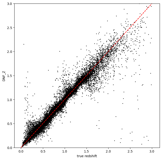
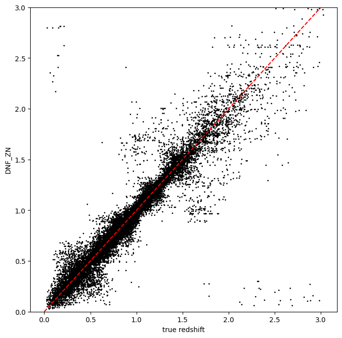
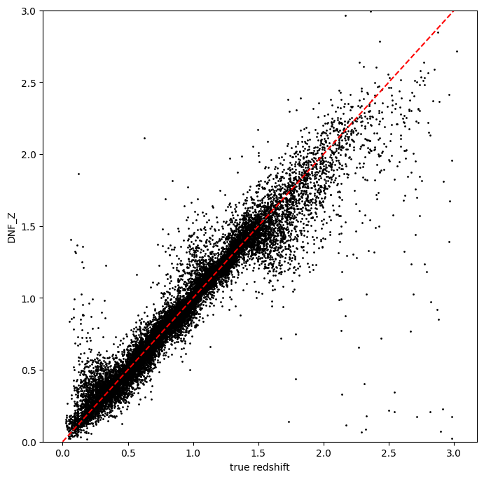
DNF calculates its own point estimate, DNF_Z, which is stored in the
qp Ensemble ancil data. Also, DNF calculates other photo-zs called
DNF_ZN.
DNF_Zrepresents the photometric redshift for each galaxy computed as the weighted average or hyperplane fit (depending on the option selected) for a set of neighbors determined by a specific metric (ENF, ANF, DNF) where the outliers are removedDNF_ZNrepresents the photometric redshift using only the closest neighbor. It is mainly used for computing the redshift distributions.
Let’s plot that versus the true redshift. We can also compute the PDF mode for each object and plot that as well:
zdnf = results.ancil["DNF_Z"].flatten()
zn_dnf = results.ancil["DNF_ZN"].flatten()
zgrid = np.linspace(0, 3, 301)
zmode = results.mode(zgrid).flatten()
zmode
array([0.08, 0.03, 0.03, ..., 3. , 2.94, 3. ], shape=(20449,))
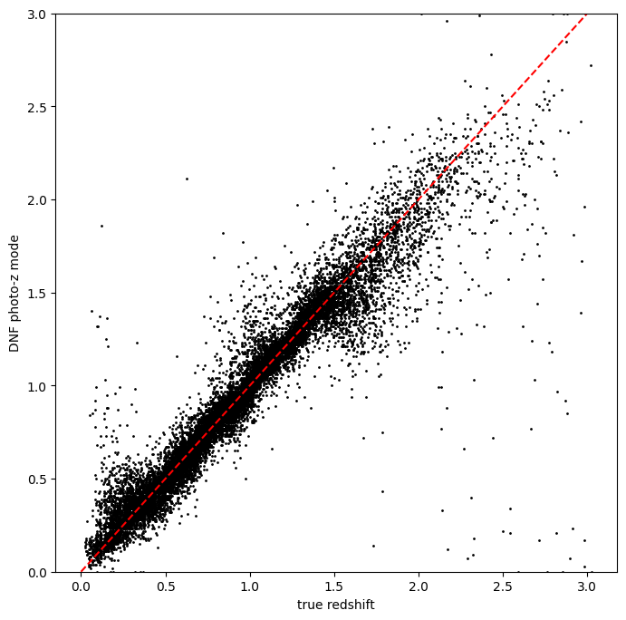
Let’s plot the redshift mode against the true redshifts to see how they look:
plt.figure(figsize=(8, 8))
plt.scatter(test_data["photometry"]["redshift"], zmode, s=1, c="k", label="DNF mode")
plt.plot([0, 3], [0, 3], "r--")
plt.xlabel("true redshift")
plt.ylabel("DNF photo-z mode")
plt.ylim(0, 3)
(0.0, 3.0)

plt.figure(figsize=(8, 8))
plt.scatter(test_data["photometry"]["redshift"], zdnf, s=1, c="k")
plt.plot([0, 3], [0, 3], "r--")
plt.xlabel("true redshift")
plt.ylabel("DNF_Z")
plt.ylim(0, 3)
(0.0, 3.0)
plt.figure(figsize=(8, 8))
plt.scatter(test_data["photometry"]["redshift"], zn_dnf, s=1, c="k")
plt.plot([0, 3], [0, 3], "r--")
plt.xlabel("true redshift")
plt.ylabel("DNF_ZN")
plt.ylim(0, 3)
(0.0, 3.0)
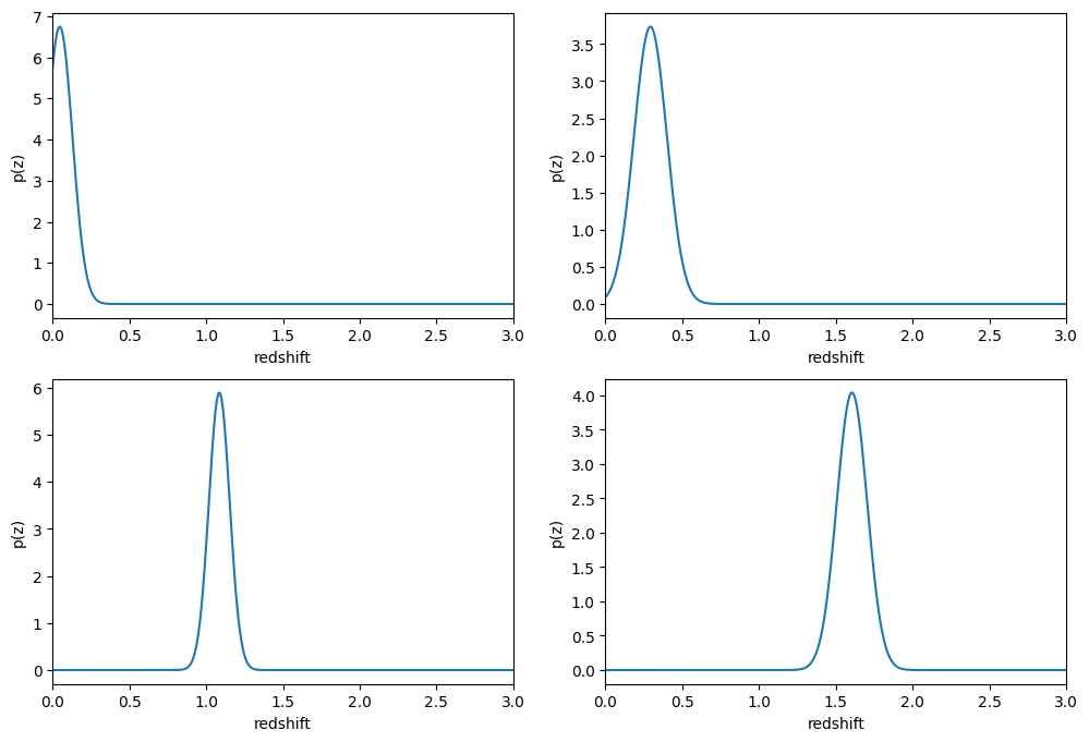
plotting PDFs
In addition to point estimates, we can also plot a few of the full PDFs
produced by DNF using the plot_native method of the qp Ensemble that
we’ve created as results. We can specify which PDF to plot with the
key argument to plot_native, let’s plot four, the 5th, 1380th,
14481st, and 18871st:
fig, axs = plt.subplots(2, 2, figsize=(12, 8))
whichgals = [4, 1379, 14480, 18870]
for ax, which in zip(axs.flat, whichgals):
    ax.set_xlim(0, 3)
    results.plot_native(key=which, axes=ax)
    ax.set_xlabel("redshift")
    ax.set_ylabel("p(z)")
Other distance metrics
Besides DNF there are options for ENF and ANF.
Let’s run our estimator using selection_mode=0 for the Euclidean
distance, and compare both the mode results and PDF results:
results2 = ri.estimation.algos.dnf.dnf_estimator(
    input_data=test_data,
    hdf5_groupname="photometry",
    model=model,
    selection_mode=0,
    nondetect_replace=True,
)
using metric ENF
Inserting handle into data store.  input: None, DNFEstimator
Inserting handle into data store.  model: {'train_mag': array([[18.040369, 16.960892, 16.653412, 16.50631 , 16.466377, 16.423904],
       [21.61559 , 20.709402, 20.533852, 20.437565, 20.408886, 20.38821 ],
       [21.851952, 20.437067, 19.709715, 19.31263 , 18.953411, 18.770441],
       ...,
       [25.185795, 24.11405 , 23.828472, 23.711334, 23.75624 , 23.83491 ],
       [26.682219, 25.068745, 24.770744, 24.587885, 24.786388, 24.673431],
       [26.926563, 25.552408, 24.984402, 24.891462, 24.842054, 24.777039]],
      shape=(10225, 6), dtype=float32), 'train_err': array([[0.00504562, 0.00500126, 0.00500058, 0.00500074, 0.0050014 ,
        0.00500337],
       [0.00955173, 0.00508365, 0.00504773, 0.00507535, 0.0051933 ,
        0.00580441],
       [0.01114765, 0.00505737, 0.00501542, 0.00501555, 0.00502286,
        0.005063  ],
       ...,
       [0.20123477, 0.01664717, 0.0122792 , 0.0153863 , 0.0272381 ,
        0.0662687 ],
       [0.7962344 , 0.03818999, 0.02692565, 0.03277681, 0.06901625,
        0.14290111],
       [0.99701214, 0.05916394, 0.03255744, 0.04307469, 0.07261812,
        0.15717329]], shape=(10225, 6), dtype=float32), 'truez': array([0.02043499, 0.01936132, 0.03672067, ..., 2.97927326, 2.98694714,
       2.97646626], shape=(10225,)), 'clf': KNeighborsRegressor(), 'train_norm': array([41.277203, 50.671963, 48.664085, ..., 58.977093, 61.49536 ,
       62.070927], shape=(10225,), dtype=float32)}, DNFEstimator
Process 0 running estimator on chunk 0 - 20,449
Process 0 estimating PZ PDF for rows 0 - 20,449
Inserting handle into data store. output: inprogress_output.hdf5, DNFEstimator
zdnf2 = results2["output"].ancil["DNF_Z"].flatten()
zgrid = np.linspace(0, 3, 301)
zmode2 = results2["output"].mode(zgrid).flatten()
plt.figure(figsize=(8, 8))
plt.scatter(test_data["photometry"]["redshift"], zmode2, s=1, c="k", label="DNF mode")
plt.plot([0, 3], [0, 3], "r--")
plt.xlabel("true redshift")
plt.ylabel("DNF photo-z mode")
plt.ylim(0, 3)
(0.0, 3.0)
plt.figure(figsize=(8, 8))
plt.scatter(test_data["photometry"]["redshift"], zdnf2, s=1, c="k")
plt.plot([0, 3], [0, 3], "r--")
plt.xlabel("true redshift")
plt.ylabel("DNF_Z")
plt.ylim(0, 3)
(0.0, 3.0)
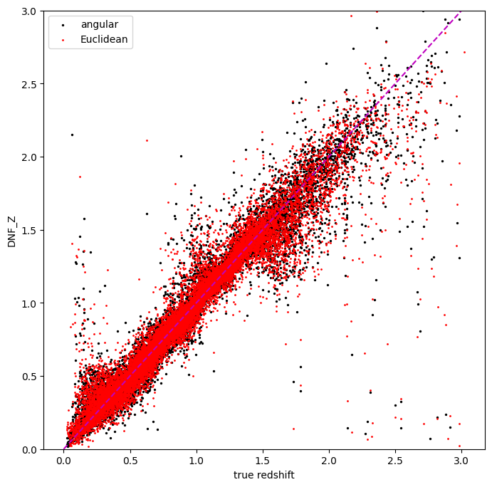
Let’s directly compare the “angular” and “Euclidean” distance estimates on the same axes:
plt.figure(figsize=(8, 8))
plt.scatter(test_data["photometry"]["redshift"], zdnf, s=2, c="k", label="angular")
plt.scatter(test_data["photometry"]["redshift"], zdnf2, s=1, c="r", label="Euclidean")
plt.legend(loc="upper left", fontsize=10)
plt.plot([0, 3], [0, 3], "m--")
plt.xlabel("true redshift")
plt.ylabel("DNF_Z")
plt.ylim(0, 3)
(0.0, 3.0)
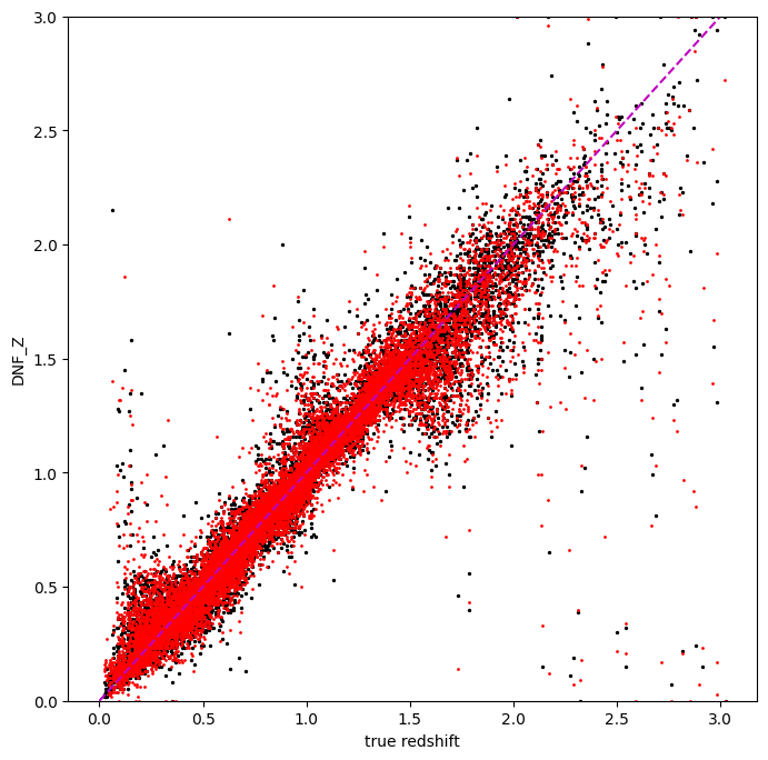
plt.figure(figsize=(8, 8))
plt.scatter(test_data["photometry"]["redshift"], zmode, s=2, c="k")
plt.scatter(test_data["photometry"]["redshift"], zmode2, s=1, c="r")
plt.plot([0, 3], [0, 3], "m--")
plt.xlabel("true redshift")
plt.ylabel("DNF_Z")
plt.ylim(0, 3)
(0.0, 3.0)
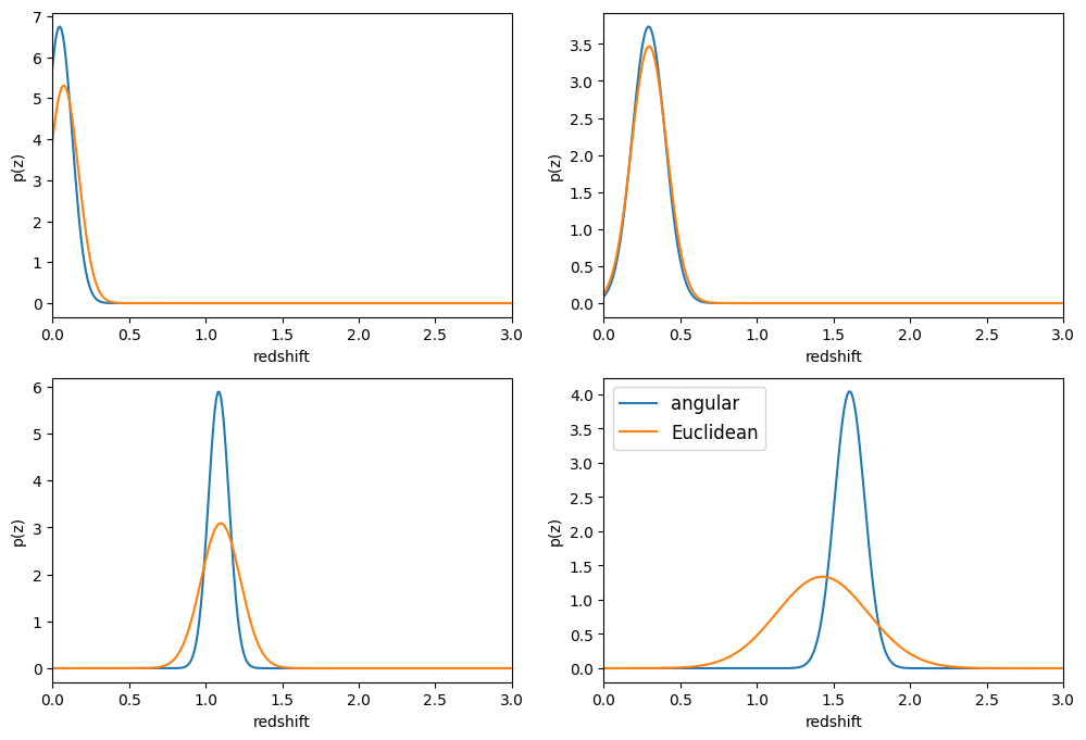
Finally, let’s directly compare the same PDFs that we plotted above
fig, axs = plt.subplots(2, 2, figsize=(12, 8))
whichgals = [4, 1379, 14480, 18870]
for ax, which in zip(axs.flat, whichgals):
    ax.set_xlim(0, 3)
    results.plot_native(key=which, axes=ax, label="angular")
    results2["output"].plot_native(key=which, axes=ax, label="Euclidean")
    ax.set_xlabel("redshift")
    ax.set_ylabel("p(z)")
ax.legend(loc="upper left", fontsize=12)
<matplotlib.legend.Legend at 0x7fc4dd5cf0d0>