i# The NZDir estimator
Author: Sam Schmidt
Last successfully run: Feb 9, 2026
Note: If you’re interested in running this in pipeline mode, see
07_NZDir.ipynb
in the pipeline_examples/estimation_examples/ folder.
This is a quick demo of the NZDir estimator, it has been ported to RAIL based on Joe Zuntz’s implementation in TXPipe here: https://github.com/LSSTDESC/TXPipe/blob/nz-dir/txpipe/nz_calibration.py
First off, let’s load the relevant packages from RAIL:
import matplotlib.pyplot as plt
import numpy as np
import pandas as pd
import rail.interactive as ri
import tables_io
from rail.utils.path_utils import find_rail_file
Install FSPS with the following commands:
pip uninstall fsps
git clone --recursive https://github.com/dfm/python-fsps.git
cd python-fsps
python -m pip install .
export SPS_HOME=$(pwd)/src/fsps/libfsps

LEPHAREDIR is being set to the default cache directory:
/home/runner/.cache/lephare/data
More than 1Gb may be written there.
LEPHAREWORK is being set to the default cache directory:
/home/runner/.cache/lephare/work
Default work cache is already linked.
This is linked to the run directory:
/home/runner/.cache/lephare/runs/20260504T123336
A module that was compiled using NumPy 1.x cannot be run in
NumPy 2.2.6 as it may crash. To support both 1.x and 2.x
versions of NumPy, modules must be compiled with NumPy 2.0.
Some module may need to rebuild instead e.g. with 'pybind11>=2.12'.

If you are a user of the module, the easiest solution will be to
downgrade to 'numpy<2' or try to upgrade the affected module.
We expect that some modules will need time to support NumPy 2.

Traceback (most recent call last):  File "/opt/hostedtoolcache/Python/3.10.20/x64/lib/python3.10/runpy.py", line 196, in _run_module_as_main
    return _run_code(code, main_globals, None,
  File "/opt/hostedtoolcache/Python/3.10.20/x64/lib/python3.10/runpy.py", line 86, in _run_code
    exec(code, run_globals)
  File "/opt/hostedtoolcache/Python/3.10.20/x64/lib/python3.10/site-packages/ipykernel_launcher.py", line 18, in <module>
    app.launch_new_instance()
  File "/opt/hostedtoolcache/Python/3.10.20/x64/lib/python3.10/site-packages/traitlets/config/application.py", line 1075, in launch_instance
    app.start()
  File "/opt/hostedtoolcache/Python/3.10.20/x64/lib/python3.10/site-packages/ipykernel/kernelapp.py", line 758, in start
    self.io_loop.start()
  File "/opt/hostedtoolcache/Python/3.10.20/x64/lib/python3.10/site-packages/tornado/platform/asyncio.py", line 211, in start
    self.asyncio_loop.run_forever()
  File "/opt/hostedtoolcache/Python/3.10.20/x64/lib/python3.10/asyncio/base_events.py", line 603, in run_forever
    self._run_once()
  File "/opt/hostedtoolcache/Python/3.10.20/x64/lib/python3.10/asyncio/base_events.py", line 1909, in _run_once
    handle._run()
  File "/opt/hostedtoolcache/Python/3.10.20/x64/lib/python3.10/asyncio/events.py", line 80, in _run
    self._context.run(self._callback, *self._args)
  File "/opt/hostedtoolcache/Python/3.10.20/x64/lib/python3.10/site-packages/ipykernel/utils.py", line 71, in preserve_context
    return await f(*args, **kwargs)
  File "/opt/hostedtoolcache/Python/3.10.20/x64/lib/python3.10/site-packages/ipykernel/kernelbase.py", line 621, in shell_main
    await self.dispatch_shell(msg, subshell_id=subshell_id)
  File "/opt/hostedtoolcache/Python/3.10.20/x64/lib/python3.10/site-packages/ipykernel/kernelbase.py", line 478, in dispatch_shell
    await result
  File "/opt/hostedtoolcache/Python/3.10.20/x64/lib/python3.10/site-packages/ipykernel/ipkernel.py", line 372, in execute_request
    await super().execute_request(stream, ident, parent)
  File "/opt/hostedtoolcache/Python/3.10.20/x64/lib/python3.10/site-packages/ipykernel/kernelbase.py", line 834, in execute_request
    reply_content = await reply_content
  File "/opt/hostedtoolcache/Python/3.10.20/x64/lib/python3.10/site-packages/ipykernel/ipkernel.py", line 464, in do_execute
    res = shell.run_cell(
  File "/opt/hostedtoolcache/Python/3.10.20/x64/lib/python3.10/site-packages/ipykernel/zmqshell.py", line 663, in run_cell
    return super().run_cell(*args, **kwargs)
  File "/opt/hostedtoolcache/Python/3.10.20/x64/lib/python3.10/site-packages/IPython/core/interactiveshell.py", line 3077, in run_cell
    result = self._run_cell(
  File "/opt/hostedtoolcache/Python/3.10.20/x64/lib/python3.10/site-packages/IPython/core/interactiveshell.py", line 3132, in _run_cell
    result = runner(coro)
  File "/opt/hostedtoolcache/Python/3.10.20/x64/lib/python3.10/site-packages/IPython/core/async_helpers.py", line 128, in _pseudo_sync_runner
    coro.send(None)
  File "/opt/hostedtoolcache/Python/3.10.20/x64/lib/python3.10/site-packages/IPython/core/interactiveshell.py", line 3336, in run_cell_async
    has_raised = await self.run_ast_nodes(code_ast.body, cell_name,
  File "/opt/hostedtoolcache/Python/3.10.20/x64/lib/python3.10/site-packages/IPython/core/interactiveshell.py", line 3519, in run_ast_nodes
    if await self.run_code(code, result, async_=asy):
  File "/opt/hostedtoolcache/Python/3.10.20/x64/lib/python3.10/site-packages/IPython/core/interactiveshell.py", line 3579, in run_code
    exec(code_obj, self.user_global_ns, self.user_ns)
  File "/tmp/ipykernel_6065/285264119.py", line 4, in <module>
    import rail.interactive as ri
  File "/opt/hostedtoolcache/Python/3.10.20/x64/lib/python3.10/site-packages/rail/interactive/__init__.py", line 3, in <module>
    from . import calib, creation, estimation, evaluation, tools
  File "/opt/hostedtoolcache/Python/3.10.20/x64/lib/python3.10/site-packages/rail/interactive/calib/__init__.py", line 3, in <module>
    from rail.utils.interactive.initialize_utils import _initialize_interactive_module
  File "/opt/hostedtoolcache/Python/3.10.20/x64/lib/python3.10/site-packages/rail/utils/interactive/initialize_utils.py", line 17, in <module>
    from rail.utils.interactive.base_utils import (
  File "/opt/hostedtoolcache/Python/3.10.20/x64/lib/python3.10/site-packages/rail/utils/interactive/base_utils.py", line 10, in <module>
    rail.stages.import_and_attach_all(silent=True)
  File "/opt/hostedtoolcache/Python/3.10.20/x64/lib/python3.10/site-packages/rail/stages/__init__.py", line 74, in import_and_attach_all
    RailEnv.import_all_packages(silent=silent)
  File "/opt/hostedtoolcache/Python/3.10.20/x64/lib/python3.10/site-packages/rail/core/introspection.py", line 541, in import_all_packages
    _imported_module = importlib.import_module(pkg)
  File "/opt/hostedtoolcache/Python/3.10.20/x64/lib/python3.10/importlib/__init__.py", line 126, in import_module
    return _bootstrap._gcd_import(name[level:], package, level)
  File "/opt/hostedtoolcache/Python/3.10.20/x64/lib/python3.10/site-packages/rail/som/__init__.py", line 1, in <module>
    from rail.creation.degraders.specz_som import *
  File "/opt/hostedtoolcache/Python/3.10.20/x64/lib/python3.10/site-packages/rail/creation/degraders/specz_som.py", line 15, in <module>
    from somoclu import Somoclu
  File "/opt/hostedtoolcache/Python/3.10.20/x64/lib/python3.10/site-packages/somoclu/__init__.py", line 11, in <module>
    from .train import Somoclu
  File "/opt/hostedtoolcache/Python/3.10.20/x64/lib/python3.10/site-packages/somoclu/train.py", line 25, in <module>
    from .somoclu_wrap import train as wrap_train
  File "/opt/hostedtoolcache/Python/3.10.20/x64/lib/python3.10/site-packages/somoclu/somoclu_wrap.py", line 11, in <module>
    import _somoclu_wrap
---------------------------------------------------------------------------

ImportError                               Traceback (most recent call last)

File /opt/hostedtoolcache/Python/3.10.20/x64/lib/python3.10/site-packages/numpy/core/_multiarray_umath.py:44, in __getattr__(attr_name)
     39     # Also print the message (with traceback).  This is because old versions
     40     # of NumPy unfortunately set up the import to replace (and hide) the
     41     # error.  The traceback shouldn't be needed, but e.g. pytest plugins
     42     # seem to swallow it and we should be failing anyway...
     43     sys.stderr.write(msg + tb_msg)
---> 44     raise ImportError(msg)
     46 ret = getattr(_multiarray_umath, attr_name, None)
     47 if ret is None:


ImportError:
A module that was compiled using NumPy 1.x cannot be run in
NumPy 2.2.6 as it may crash. To support both 1.x and 2.x
versions of NumPy, modules must be compiled with NumPy 2.0.
Some module may need to rebuild instead e.g. with 'pybind11>=2.12'.

If you are a user of the module, the easiest solution will be to
downgrade to 'numpy<2' or try to upgrade the affected module.
We expect that some modules will need time to support NumPy 2.
Warning: the binary library cannot be imported. You cannot train maps, but you can load and analyze ones that you have already saved.
The problem occurs because either compilation failed when you installed Somoclu or a path is missing from the dependencies when you are trying to import it. Please refer to the documentation to see your options.
test_dc2_training_9816.hdf5 contains ~10,000 galaxies from healpix
9816 of the cosmoDC2 “truth” catalog, and the “validation” data set
contains ~20,000 galaxies from this same healpix pixel.
trainFile = find_rail_file("examples_data/testdata/test_dc2_training_9816.hdf5")
testFile = find_rail_file("examples_data/testdata/test_dc2_validation_9816.hdf5")
training_data = tables_io.read(trainFile)
Let’s read test data in with tables_io, and then split it up into several tomographic bins. We can mock up some simple “tomographic” bins via their true redshift. The degrader expects a pandas DataFrame, so we will create three dataframes for each of a low, mid, and hi redshift sample. Let’s also add a weight column to the test data while we are at it, this will be used later by the NZDir algorithm (for now we’ll set all weights to one):
rawdata = tables_io.read(testFile)["photometry"]
df = tables_io.convert(rawdata, tType=tables_io.types.PD_DATAFRAME)
szcol = rawdata["redshift"]
numintest = len(szcol)
df["weight"] = np.ones(numintest, dtype="float")
lowmask = szcol <= 0.75
midmask = np.logical_and(szcol > 0.75, szcol < 1.25)
himask = szcol >= 1.25
low_bin = df[lowmask]
mid_bin = df[midmask]
hi_bin = df[himask]
The algorithm:
The NZDir estimator tries to reconstruct the redshift distribution for an unknown sample (which we’ll alternately call the “photometric sample”, as it has photometric, but not spectroscopic information for each galaxy) by finding spectroscopic galaxies with similar magnitudes/colors and assigning a redshift based on those similarly-colored objects.
In practice, this particular algorithm actually reverses that process:
it defines a neighborhood around each spectroscopic object (based on the
distance to the Nth nearest neighbor, where N is defined by the user via
the parameter n_neigh). Then, it loops over the set of all
spectroscopic objects and adds its (weighted) redshift to a histogram
for each photometric object that it finds within the annulus.
This process is more efficient computationally, and has the benefit of automatically “ignoring” photometric objects that have no similarly colored spectroscopic objects nearby. However, that could also be seen as a limitation, as if there are areas of color^N space not covered by your training sample, those galaxies will be “skipped” when assembling the tomographic redshift N(z) estimate, which can lead to biased results, as we will show later in this demo.
Like PDF estimators, the algorithm is broken up into an “inform” stage and an “estimate” stage. The inform stage creates the neighbors for the spectroscopic samples and calculates the distance to the Nth nearest neighbor that is used to determine annulus checks around each spec-z object. These quantites are stored in a specified model file that is loaded and used by the estimate stage.
Let’s also add a “weight column” to the training data to test functionality. For simplicity we already set the weights to 1.0 for all photometric galaxies a few cells above, and now let’s set weights of 0.5 for all spectroscopic galaxies. This should have no impact on the recovery compared to having no weights included. Note that if weights are not included, the algorithm will set all weights to 1.0. However, these weights could be used in more realistic analyses to reweight training or test samples to account for various biases.
numinphot = len(training_data["photometry"]["redshift"])
training_data["photometry"]["weight"] = np.ones(numinphot, dtype="float") * 0.5
zmin = 0.0
zmax = 3.0
xmanybins = 25
Now, let’s set up or estimator, first creating a stage for the informer.
We define any input variables in a dictionary and then use that with
make_stage to create an instance of our NZDirSummarizer. We’ll
create a histogram of 25 bins, using 5 nearest neighbors to define our
specz neighborhood, and above we defined our bin column as “bin”:
nzdir_model = ri.estimation.algos.nz_dir.nz_dir_informer(
    training_data=training_data,
    n_neigh=5,
    szweightcol="weight",
)["model"]
Inserting handle into data store.  input: None, NZDirInformer
Inserting handle into data store.  model: inprogress_model.pkl, NZDirInformer
Now, let’s set up our NZDir estimator, providing parameters for the
redshift grid, photomtetric weight column, and the model that we created
with the informer. Note that NZDir returns N bootstrap samples rather
than just a single distribution. The code draws bootstrap samples from
the spectroscopic sample to use as input as the training data.
nsamples can be used to set the number of bootstrap samples
returned, for this demo we will only generate 20:
summdict = dict(
    leafsize=20,
    zmin=zmin,
    zmax=zmax,
    nzbins=xmanybins,
    nsamples=20,
    phot_weightcol="weight",
    model=nzdir_model,
    hdf5_groupname="",
)
We have three tomographic bins, we can make a stage and run each one in
a loop. To run our Nz Estimator we just need to run estimate with
arguments for the test and training data handles as named in the Data
Store: The code uses a fast Nearest Neighbor calculation and KDTree
calculation, so this should run very fast:
%%time
bin_ens = {}
binnames = ["low", "mid", "hi"]
bin_datasets = [low_bin, mid_bin, hi_bin]
for bin, indata in zip(binnames, bin_datasets):
    bin_ens[f"{bin}"] = ri.estimation.algos.nz_dir.nz_dir_summarizer(
        input_data=indata, **summdict
    )["output"]
Inserting handle into data store.  input: None, NZDirSummarizer
Inserting handle into data store.  model: {'distances': array([2.51892877, 0.85703786, 0.48703015, ..., 0.49684775, 0.49851571,
       0.30138747], shape=(10225,)), 'szusecols': ['mag_u_lsst', 'mag_g_lsst', 'mag_r_lsst', 'mag_i_lsst', 'mag_z_lsst', 'mag_y_lsst'], 'szweights': array([0.5, 0.5, 0.5, ..., 0.5, 0.5, 0.5], shape=(10225,)), 'szvec': array([0.02043499, 0.01936132, 0.03672067, ..., 2.97927326, 2.98694714,
       2.97646626], shape=(10225,)), 'sz_mag_data': array([[18.040369, 16.960892, 16.653412, 16.50631 , 16.466377, 16.423904],
       [21.61559 , 20.709402, 20.533852, 20.437565, 20.408886, 20.38821 ],
       [21.851952, 20.437067, 19.709715, 19.31263 , 18.953411, 18.770441],
       ...,
       [25.185795, 24.11405 , 23.828472, 23.711334, 23.75624 , 23.83491 ],
       [26.682219, 25.068745, 24.770744, 24.587885, 24.786388, 24.673431],
       [26.926563, 25.552408, 24.984402, 24.891462, 24.842054, 24.777039]],
      shape=(10225, 6), dtype=float32)}, NZDirSummarizer
Process 0 running estimator on chunk 0 - 7679
Inserting handle into data store.  single_NZ: inprogress_single_NZ.hdf5, NZDirSummarizer
Inserting handle into data store.  output: inprogress_output.hdf5, NZDirSummarizer
Inserting handle into data store.  input: None, NZDirSummarizer
Inserting handle into data store.  model: {'distances': array([2.51892877, 0.85703786, 0.48703015, ..., 0.49684775, 0.49851571,
       0.30138747], shape=(10225,)), 'szusecols': ['mag_u_lsst', 'mag_g_lsst', 'mag_r_lsst', 'mag_i_lsst', 'mag_z_lsst', 'mag_y_lsst'], 'szweights': array([0.5, 0.5, 0.5, ..., 0.5, 0.5, 0.5], shape=(10225,)), 'szvec': array([0.02043499, 0.01936132, 0.03672067, ..., 2.97927326, 2.98694714,
       2.97646626], shape=(10225,)), 'sz_mag_data': array([[18.040369, 16.960892, 16.653412, 16.50631 , 16.466377, 16.423904],
       [21.61559 , 20.709402, 20.533852, 20.437565, 20.408886, 20.38821 ],
       [21.851952, 20.437067, 19.709715, 19.31263 , 18.953411, 18.770441],
       ...,
       [25.185795, 24.11405 , 23.828472, 23.711334, 23.75624 , 23.83491 ],
       [26.682219, 25.068745, 24.770744, 24.587885, 24.786388, 24.673431],
       [26.926563, 25.552408, 24.984402, 24.891462, 24.842054, 24.777039]],
      shape=(10225, 6), dtype=float32)}, NZDirSummarizer
Process 0 running estimator on chunk 0 - 8513
Inserting handle into data store.  single_NZ: inprogress_single_NZ.hdf5, NZDirSummarizer
Inserting handle into data store.  output: inprogress_output.hdf5, NZDirSummarizer
Inserting handle into data store.  input: None, NZDirSummarizer
Inserting handle into data store.  model: {'distances': array([2.51892877, 0.85703786, 0.48703015, ..., 0.49684775, 0.49851571,
       0.30138747], shape=(10225,)), 'szusecols': ['mag_u_lsst', 'mag_g_lsst', 'mag_r_lsst', 'mag_i_lsst', 'mag_z_lsst', 'mag_y_lsst'], 'szweights': array([0.5, 0.5, 0.5, ..., 0.5, 0.5, 0.5], shape=(10225,)), 'szvec': array([0.02043499, 0.01936132, 0.03672067, ..., 2.97927326, 2.98694714,
       2.97646626], shape=(10225,)), 'sz_mag_data': array([[18.040369, 16.960892, 16.653412, 16.50631 , 16.466377, 16.423904],
       [21.61559 , 20.709402, 20.533852, 20.437565, 20.408886, 20.38821 ],
       [21.851952, 20.437067, 19.709715, 19.31263 , 18.953411, 18.770441],
       ...,
       [25.185795, 24.11405 , 23.828472, 23.711334, 23.75624 , 23.83491 ],
       [26.682219, 25.068745, 24.770744, 24.587885, 24.786388, 24.673431],
       [26.926563, 25.552408, 24.984402, 24.891462, 24.842054, 24.777039]],
      shape=(10225, 6), dtype=float32)}, NZDirSummarizer
Process 0 running estimator on chunk 0 - 4257
Inserting handle into data store.  single_NZ: inprogress_single_NZ.hdf5, NZDirSummarizer
Inserting handle into data store.  output: inprogress_output.hdf5, NZDirSummarizer
CPU times: user 243 ms, sys: 3.72 ms, total: 246 ms
Wall time: 245 ms
indeed, for our 20,000 test and 10,000 training galaxies, it takes less than a second to run all three bins! Now, let’s plot our estimates and compare to the true distributions in our tomo bins. While the ensembles actually contain 20 distributions, we will plot only the first bootstrap realization for each bin:
samebins = np.linspace(zmin, zmax, xmanybins)
binsize = samebins[1] - samebins[0]
bincents = 0.5 * (samebins[1:] + samebins[:-1])

fig, axs = plt.subplots(1, 3, figsize=(20, 6))
bin_datasets = [low_bin, mid_bin, hi_bin]
binnames = ["low", "mid", "hi"]
for ii, (bin, indata) in enumerate(zip(binnames, bin_datasets)):
    truehist, bins = np.histogram(indata["redshift"], bins=samebins)
    norm = np.sum(truehist) * binsize
    truehist = np.array(truehist) / norm
    bin_ens[f"{bin}"].plot_native(axes=axs[ii], label="DIR estimate")
    axs[ii].bar(
        bincents,
        truehist,
        alpha=0.55,
        width=binsize,
        color="b",
        label="true redshift distn",
    )
plt.legend(loc="upper right", fontsize=12)
plt.title("representative training data", fontsize=15)
plt.xlabel("redshift", fontsize=12)
plt.ylabel("N(z)", fontsize=12)
Text(0, 0.5, 'N(z)')
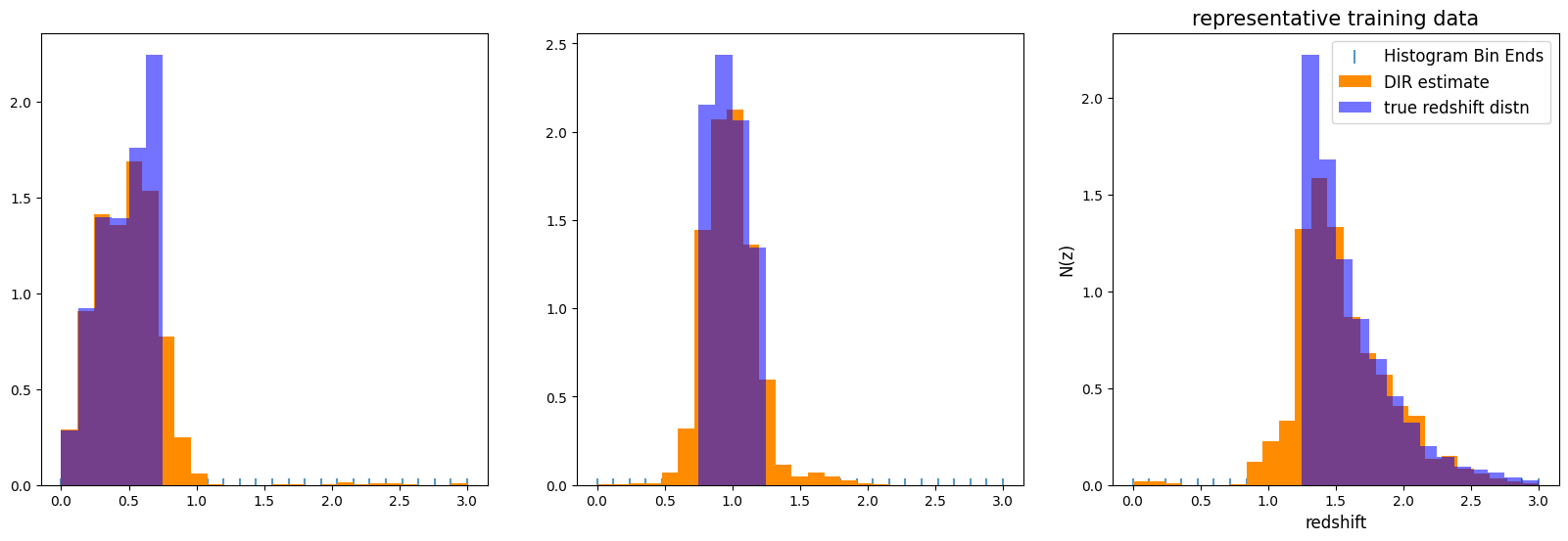
Non-representative data
That looks very nice, while there is a little bit of “slosh” outside of each bin, we have a relatively compact and accurate representation from the DIR method! This makes sense, as our training and test data are drawn from the same underlying distribution (in this case cosmoDC2_v1.1.4). However, how will things look if we are missing chunks of data, or have incorrect redshifts in our spec-z sample? We can use RAIL’s degradation modules to do just that: place incorrect redshifts for percentage of the training data, and we can make a magnitude cut that will limite the redshift and color range of our training data:
Let’s import the necessary modules from rail.creation.degraders, we will put in “line confusion” for 5% of our sample, and then cut the sample at magnitude 23.5:
The degrader expects a pandas dataframe, so let’s construct one and add it to the data store, we’ll strip out the ‘photometry’ hdf5 while we’re at it:
degrade_data = pd.DataFrame(training_data["photometry"])
Now, apply our degraders:
train_data_conf = ri.creation.degraders.spectroscopic_degraders.line_confusion(
    sample=degrade_data,
    hdf5_groupname="photometry",
    true_wavelen=5007.0,
    wrong_wavelen=3727.0,
    frac_wrong=0.05,
)["output"]

train_data_cut = ri.creation.degraders.quantityCut.quantity_cut(
    sample=train_data_conf, hdf5_groupname="photometry", cuts={"mag_i_lsst": 23.5}
)
Inserting handle into data store.  input: None, LineConfusion
Inserting handle into data store.  output: inprogress_output.pq, LineConfusion
Inserting handle into data store.  input: None, QuantityCut
Inserting handle into data store.  output: inprogress_output.pq, QuantityCut
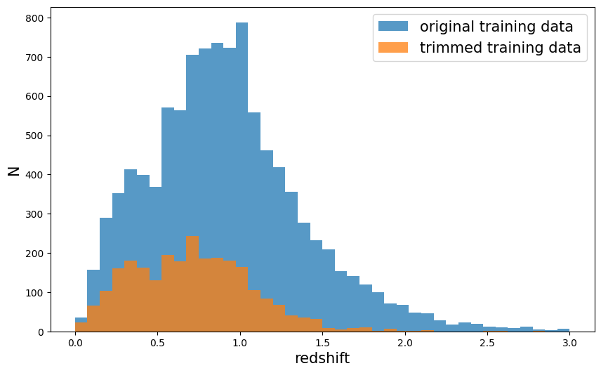
Let’s plot our trimmed training sample, we see that we have fewer galaxies, so we’ll be subject to more “shot noise”/discretization of the redshifts, and we are very incomplete at high redshift.
# compare original specz data to degraded data
fig = plt.figure(figsize=(10, 6))
xbins = np.linspace(0, 3, 41)
plt.hist(
    training_data["photometry"]["redshift"],
    bins=xbins,
    alpha=0.75,
    label="original training data",
)
plt.hist(
    train_data_cut["output"]["redshift"],
    bins=xbins,
    alpha=0.75,
    label="trimmed training data",
)
plt.legend(loc="upper right", fontsize=15)
plt.xlabel("redshift", fontsize=15)
plt.ylabel("N", fontsize=15)
Text(0, 0.5, 'N')
Let’s re-run our estimator on the same test data but now with our incomplete training data:
xinformdict = dict(
    n_neigh=5,
    bincol="bin",
    szweightcol="weight",
    hdf5_groupname="",
)
newsumm_model = ri.estimation.algos.nz_dir.nz_dir_informer(
    training_data=train_data_cut["output"], **xinformdict
)["model"]
Inserting handle into data store.  input: None, NZDirInformer
Inserting handle into data store.  model: inprogress_model.pkl, NZDirInformer
Now we need to re-run our tomographic bin estimates with this new model:
%%time
xestimatedict = dict(
    leafsize=20,
    zmin=zmin,
    zmax=zmax,
    nzbins=xmanybins,
    hdf5_groupname="",
    nsamples=20,
    phot_weightcol="weight",
    model=newsumm_model,
)
new_ens = {}
binnames = ["low", "mid", "hi"]
bin_datasets = [low_bin, mid_bin, hi_bin]
for bin, indata in zip(binnames, bin_datasets):
    new_ens[f"{bin}"] = ri.estimation.algos.nz_dir.nz_dir_summarizer(
        input_data=indata, **xestimatedict
    )["output"]
Inserting handle into data store.  input: None, NZDirSummarizer
Inserting handle into data store.  model: {'distances': array([2.51892877, 0.85703786, 0.48703015, ..., 0.6715168 , 0.64272626,
       0.77295267], shape=(2576,)), 'szusecols': ['mag_u_lsst', 'mag_g_lsst', 'mag_r_lsst', 'mag_i_lsst', 'mag_z_lsst', 'mag_y_lsst'], 'szweights': array([0.5, 0.5, 0.5, ..., 0.5, 0.5, 0.5], shape=(2576,)), 'szvec': array([0.02043499, 0.01936132, 0.03672067, ..., 2.54900666, 2.60658155,
       2.79650929], shape=(2576,)), 'sz_mag_data': array([[18.04036903, 16.96089172, 16.65341187, 16.50630951, 16.46637726,
        16.42390442],
       [21.61558914, 20.70940208, 20.53385162, 20.43756485, 20.40888596,
        20.3882103 ],
       [21.8519516 , 20.43706703, 19.70971489, 19.3126297 , 18.9534111 ,
        18.77044106],
       ...,
       [24.30592918, 23.65139198, 23.47483635, 23.44481087, 23.51615524,
        23.43613243],
       [24.01694679, 23.49385071, 23.38884163, 23.35801315, 23.45185089,
        23.43612099],
       [24.16078758, 23.40859985, 23.29878235, 23.29213524, 23.34983253,
        23.5138588 ]], shape=(2576, 6))}, NZDirSummarizer
Process 0 running estimator on chunk 0 - 7679
Inserting handle into data store.  single_NZ: inprogress_single_NZ.hdf5, NZDirSummarizer
Inserting handle into data store.  output: inprogress_output.hdf5, NZDirSummarizer
Inserting handle into data store.  input: None, NZDirSummarizer
Inserting handle into data store.  model: {'distances': array([2.51892877, 0.85703786, 0.48703015, ..., 0.6715168 , 0.64272626,
       0.77295267], shape=(2576,)), 'szusecols': ['mag_u_lsst', 'mag_g_lsst', 'mag_r_lsst', 'mag_i_lsst', 'mag_z_lsst', 'mag_y_lsst'], 'szweights': array([0.5, 0.5, 0.5, ..., 0.5, 0.5, 0.5], shape=(2576,)), 'szvec': array([0.02043499, 0.01936132, 0.03672067, ..., 2.54900666, 2.60658155,
       2.79650929], shape=(2576,)), 'sz_mag_data': array([[18.04036903, 16.96089172, 16.65341187, 16.50630951, 16.46637726,
        16.42390442],
       [21.61558914, 20.70940208, 20.53385162, 20.43756485, 20.40888596,
        20.3882103 ],
       [21.8519516 , 20.43706703, 19.70971489, 19.3126297 , 18.9534111 ,
        18.77044106],
       ...,
       [24.30592918, 23.65139198, 23.47483635, 23.44481087, 23.51615524,
        23.43613243],
       [24.01694679, 23.49385071, 23.38884163, 23.35801315, 23.45185089,
        23.43612099],
       [24.16078758, 23.40859985, 23.29878235, 23.29213524, 23.34983253,
        23.5138588 ]], shape=(2576, 6))}, NZDirSummarizer
Process 0 running estimator on chunk 0 - 8513
Inserting handle into data store.  single_NZ: inprogress_single_NZ.hdf5, NZDirSummarizer
Inserting handle into data store.  output: inprogress_output.hdf5, NZDirSummarizer
Inserting handle into data store.  input: None, NZDirSummarizer
Inserting handle into data store.  model: {'distances': array([2.51892877, 0.85703786, 0.48703015, ..., 0.6715168 , 0.64272626,
       0.77295267], shape=(2576,)), 'szusecols': ['mag_u_lsst', 'mag_g_lsst', 'mag_r_lsst', 'mag_i_lsst', 'mag_z_lsst', 'mag_y_lsst'], 'szweights': array([0.5, 0.5, 0.5, ..., 0.5, 0.5, 0.5], shape=(2576,)), 'szvec': array([0.02043499, 0.01936132, 0.03672067, ..., 2.54900666, 2.60658155,
       2.79650929], shape=(2576,)), 'sz_mag_data': array([[18.04036903, 16.96089172, 16.65341187, 16.50630951, 16.46637726,
        16.42390442],
       [21.61558914, 20.70940208, 20.53385162, 20.43756485, 20.40888596,
        20.3882103 ],
       [21.8519516 , 20.43706703, 19.70971489, 19.3126297 , 18.9534111 ,
        18.77044106],
       ...,
       [24.30592918, 23.65139198, 23.47483635, 23.44481087, 23.51615524,
        23.43613243],
       [24.01694679, 23.49385071, 23.38884163, 23.35801315, 23.45185089,
        23.43612099],
       [24.16078758, 23.40859985, 23.29878235, 23.29213524, 23.34983253,
        23.5138588 ]], shape=(2576, 6))}, NZDirSummarizer
Process 0 running estimator on chunk 0 - 4257
Inserting handle into data store.  single_NZ: inprogress_single_NZ.hdf5, NZDirSummarizer
Inserting handle into data store.  output: inprogress_output.hdf5, NZDirSummarizer
CPU times: user 74.4 ms, sys: 938 μs, total: 75.4 ms
Wall time: 75.1 ms
fig, axs = plt.subplots(1, 3, figsize=(20, 6))
samebins = np.linspace(0, 3, xmanybins)
binsize = samebins[1] - samebins[0]
bincents = 0.5 * (samebins[1:] + samebins[:-1])
bin_datasets = [low_bin, mid_bin, hi_bin]
binnames = ["low", "mid", "hi"]

for ii, (bin, indata) in enumerate(zip(binnames, bin_datasets)):
    truehist, bins = np.histogram(indata["redshift"], bins=samebins)
    norm = np.sum(truehist) * binsize
    truehist = np.array(truehist) / norm
    new_ens[f"{bin}"].plot_native(axes=axs[ii], label="DIR estimate")
    axs[ii].bar(
        bincents,
        truehist,
        alpha=0.55,
        width=binsize,
        color="b",
        label="true redshift distn",
    )
axs[0].legend(loc="upper right", fontsize=12)
axs[1].set_title("non-representative training data", fontsize=15)
axs[1].set_xlabel("redshift", fontsize=15)
axs[0].set_ylabel("N(z)", fontsize=15)
Text(0, 0.5, 'N(z)')
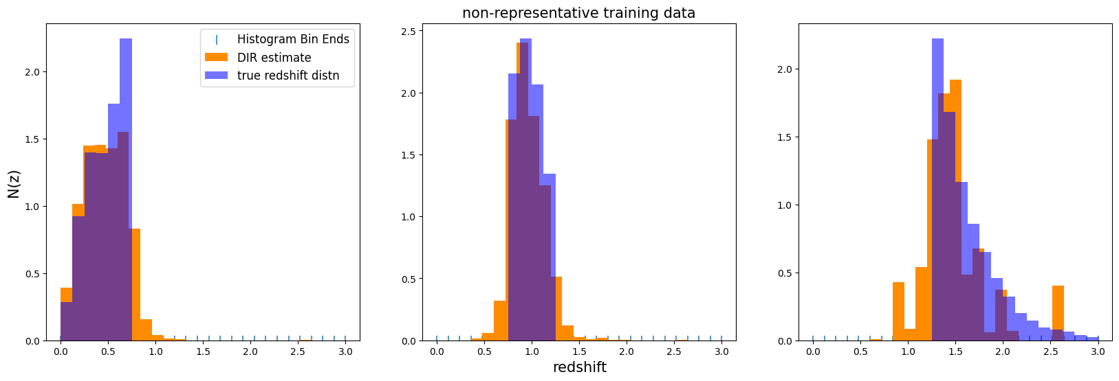
We see that the high redshift bin, where our training set was very incomplete, looks particularly bad, as expected. Bins 1 and 2 look surprisingly good, which is a promising sign that, even when a brighter magnitude cut is enforced, this method is sometimes still able to produce reasonable results.