Test Sampled Summarizers

Author: Sam Schmidt

Last successfully run: Feb 9, 2026

June 28 update: I modified the summarizers to output not just N sample N(z) distributions (saved to the file specified via the output keyword), but also the single fiducial N(z) estimate (saved to the file specified via the single_NZ keyword). I also updated NZDir and included it in this example notebook

Note: If you’re interested in running this in pipeline mode, see 13_Sampled_Summarizers.ipynb in the pipeline_examples/estimation_examples/ folder.

import matplotlib.pyplot as plt
import numpy as np
import rail.interactive as ri
import tables_io
from rail.utils.path_utils import find_rail_file

Install FSPS with the following commands:
pip uninstall fsps
git clone --recursive https://github.com/dfm/python-fsps.git
cd python-fsps
python -m pip install .
export SPS_HOME=$(pwd)/src/fsps/libfsps

LEPHAREDIR is being set to the default cache directory:
/home/runner/.cache/lephare/data
More than 1Gb may be written there.
LEPHAREWORK is being set to the default cache directory:
/home/runner/.cache/lephare/work
Default work cache is already linked.
This is linked to the run directory:
/home/runner/.cache/lephare/runs/20260504T123336

A module that was compiled using NumPy 1.x cannot be run in
NumPy 2.2.6 as it may crash. To support both 1.x and 2.x
versions of NumPy, modules must be compiled with NumPy 2.0.
Some module may need to rebuild instead e.g. with 'pybind11>=2.12'.

If you are a user of the module, the easiest solution will be to
downgrade to 'numpy<2' or try to upgrade the affected module.
We expect that some modules will need time to support NumPy 2.

Traceback (most recent call last):  File "/opt/hostedtoolcache/Python/3.10.20/x64/lib/python3.10/runpy.py", line 196, in _run_module_as_main
    return _run_code(code, main_globals, None,
  File "/opt/hostedtoolcache/Python/3.10.20/x64/lib/python3.10/runpy.py", line 86, in _run_code
    exec(code, run_globals)
  File "/opt/hostedtoolcache/Python/3.10.20/x64/lib/python3.10/site-packages/ipykernel_launcher.py", line 18, in <module>
    app.launch_new_instance()
  File "/opt/hostedtoolcache/Python/3.10.20/x64/lib/python3.10/site-packages/traitlets/config/application.py", line 1075, in launch_instance
    app.start()
  File "/opt/hostedtoolcache/Python/3.10.20/x64/lib/python3.10/site-packages/ipykernel/kernelapp.py", line 758, in start
    self.io_loop.start()
  File "/opt/hostedtoolcache/Python/3.10.20/x64/lib/python3.10/site-packages/tornado/platform/asyncio.py", line 211, in start
    self.asyncio_loop.run_forever()
  File "/opt/hostedtoolcache/Python/3.10.20/x64/lib/python3.10/asyncio/base_events.py", line 603, in run_forever
    self._run_once()
  File "/opt/hostedtoolcache/Python/3.10.20/x64/lib/python3.10/asyncio/base_events.py", line 1909, in _run_once
    handle._run()
  File "/opt/hostedtoolcache/Python/3.10.20/x64/lib/python3.10/asyncio/events.py", line 80, in _run
    self._context.run(self._callback, *self._args)
  File "/opt/hostedtoolcache/Python/3.10.20/x64/lib/python3.10/site-packages/ipykernel/utils.py", line 71, in preserve_context
    return await f(*args, **kwargs)
  File "/opt/hostedtoolcache/Python/3.10.20/x64/lib/python3.10/site-packages/ipykernel/kernelbase.py", line 621, in shell_main
    await self.dispatch_shell(msg, subshell_id=subshell_id)
  File "/opt/hostedtoolcache/Python/3.10.20/x64/lib/python3.10/site-packages/ipykernel/kernelbase.py", line 478, in dispatch_shell
    await result
  File "/opt/hostedtoolcache/Python/3.10.20/x64/lib/python3.10/site-packages/ipykernel/ipkernel.py", line 372, in execute_request
    await super().execute_request(stream, ident, parent)
  File "/opt/hostedtoolcache/Python/3.10.20/x64/lib/python3.10/site-packages/ipykernel/kernelbase.py", line 834, in execute_request
    reply_content = await reply_content
  File "/opt/hostedtoolcache/Python/3.10.20/x64/lib/python3.10/site-packages/ipykernel/ipkernel.py", line 464, in do_execute
    res = shell.run_cell(
  File "/opt/hostedtoolcache/Python/3.10.20/x64/lib/python3.10/site-packages/ipykernel/zmqshell.py", line 663, in run_cell
    return super().run_cell(*args, **kwargs)
  File "/opt/hostedtoolcache/Python/3.10.20/x64/lib/python3.10/site-packages/IPython/core/interactiveshell.py", line 3077, in run_cell
    result = self._run_cell(
  File "/opt/hostedtoolcache/Python/3.10.20/x64/lib/python3.10/site-packages/IPython/core/interactiveshell.py", line 3132, in _run_cell
    result = runner(coro)
  File "/opt/hostedtoolcache/Python/3.10.20/x64/lib/python3.10/site-packages/IPython/core/async_helpers.py", line 128, in _pseudo_sync_runner
    coro.send(None)
  File "/opt/hostedtoolcache/Python/3.10.20/x64/lib/python3.10/site-packages/IPython/core/interactiveshell.py", line 3336, in run_cell_async
    has_raised = await self.run_ast_nodes(code_ast.body, cell_name,
  File "/opt/hostedtoolcache/Python/3.10.20/x64/lib/python3.10/site-packages/IPython/core/interactiveshell.py", line 3519, in run_ast_nodes
    if await self.run_code(code, result, async_=asy):
  File "/opt/hostedtoolcache/Python/3.10.20/x64/lib/python3.10/site-packages/IPython/core/interactiveshell.py", line 3579, in run_code
    exec(code_obj, self.user_global_ns, self.user_ns)
  File "/tmp/ipykernel_5906/4087826718.py", line 3, in <module>
    import rail.interactive as ri
  File "/opt/hostedtoolcache/Python/3.10.20/x64/lib/python3.10/site-packages/rail/interactive/__init__.py", line 3, in <module>
    from . import calib, creation, estimation, evaluation, tools
  File "/opt/hostedtoolcache/Python/3.10.20/x64/lib/python3.10/site-packages/rail/interactive/calib/__init__.py", line 3, in <module>
    from rail.utils.interactive.initialize_utils import _initialize_interactive_module
  File "/opt/hostedtoolcache/Python/3.10.20/x64/lib/python3.10/site-packages/rail/utils/interactive/initialize_utils.py", line 17, in <module>
    from rail.utils.interactive.base_utils import (
  File "/opt/hostedtoolcache/Python/3.10.20/x64/lib/python3.10/site-packages/rail/utils/interactive/base_utils.py", line 10, in <module>
    rail.stages.import_and_attach_all(silent=True)
  File "/opt/hostedtoolcache/Python/3.10.20/x64/lib/python3.10/site-packages/rail/stages/__init__.py", line 74, in import_and_attach_all
    RailEnv.import_all_packages(silent=silent)
  File "/opt/hostedtoolcache/Python/3.10.20/x64/lib/python3.10/site-packages/rail/core/introspection.py", line 541, in import_all_packages
    _imported_module = importlib.import_module(pkg)
  File "/opt/hostedtoolcache/Python/3.10.20/x64/lib/python3.10/importlib/__init__.py", line 126, in import_module
    return _bootstrap._gcd_import(name[level:], package, level)
  File "/opt/hostedtoolcache/Python/3.10.20/x64/lib/python3.10/site-packages/rail/som/__init__.py", line 1, in <module>
    from rail.creation.degraders.specz_som import *
  File "/opt/hostedtoolcache/Python/3.10.20/x64/lib/python3.10/site-packages/rail/creation/degraders/specz_som.py", line 15, in <module>
    from somoclu import Somoclu
  File "/opt/hostedtoolcache/Python/3.10.20/x64/lib/python3.10/site-packages/somoclu/__init__.py", line 11, in <module>
    from .train import Somoclu
  File "/opt/hostedtoolcache/Python/3.10.20/x64/lib/python3.10/site-packages/somoclu/train.py", line 25, in <module>
    from .somoclu_wrap import train as wrap_train
  File "/opt/hostedtoolcache/Python/3.10.20/x64/lib/python3.10/site-packages/somoclu/somoclu_wrap.py", line 11, in <module>
    import _somoclu_wrap

---------------------------------------------------------------------------

ImportError                               Traceback (most recent call last)

File /opt/hostedtoolcache/Python/3.10.20/x64/lib/python3.10/site-packages/numpy/core/_multiarray_umath.py:44, in __getattr__(attr_name)
     39     # Also print the message (with traceback).  This is because old versions
     40     # of NumPy unfortunately set up the import to replace (and hide) the
     41     # error.  The traceback shouldn't be needed, but e.g. pytest plugins
     42     # seem to swallow it and we should be failing anyway...
     43     sys.stderr.write(msg + tb_msg)
---> 44     raise ImportError(msg)
     46 ret = getattr(_multiarray_umath, attr_name, None)
     47 if ret is None:


ImportError:
A module that was compiled using NumPy 1.x cannot be run in
NumPy 2.2.6 as it may crash. To support both 1.x and 2.x
versions of NumPy, modules must be compiled with NumPy 2.0.
Some module may need to rebuild instead e.g. with 'pybind11>=2.12'.

If you are a user of the module, the easiest solution will be to
downgrade to 'numpy<2' or try to upgrade the affected module.
We expect that some modules will need time to support NumPy 2.

Warning: the binary library cannot be imported. You cannot train maps, but you can load and analyze ones that you have already saved.
The problem occurs because either compilation failed when you installed Somoclu or a path is missing from the dependencies when you are trying to import it. Please refer to the documentation to see your options.

To create some N(z) distributions, we’ll want some PDFs to work with first, for a quick demo let’s just run some photo-z’s using the KNearNeighEstimator estimator using the 10,000 training galaxies to generate ~20,000 PDFs using data from healpix 9816 of cosmoDC2_v1.1.4 that are included in the RAIL repo:

knn_dict = dict(
    zmin=0.0,
    zmax=3.0,
    nzbins=301,
    trainfrac=0.75,
    sigma_grid_min=0.01,
    sigma_grid_max=0.07,
    ngrid_sigma=10,
    nneigh_min=3,
    nneigh_max=7,
    hdf5_groupname="photometry",
)

trainFile = find_rail_file("examples_data/testdata/test_dc2_training_9816.hdf5")
testFile = find_rail_file("examples_data/testdata/test_dc2_validation_9816.hdf5")
training_data = tables_io.read(trainFile)
test_data = tables_io.read(testFile)

# train knnpz
model = ri.estimation.algos.k_nearneigh.k_near_neigh_informer(
    training_data=training_data, **knn_dict
)["model"]

Inserting handle into data store.  input: None, KNearNeighInformer
split into 7669 training and 2556 validation samples
finding best fit sigma and NNeigh...

best fit values are sigma=0.023333333333333334 and numneigh=7



Inserting handle into data store.  model: inprogress_model.pkl, KNearNeighInformer

qp_data = ri.estimation.algos.k_nearneigh.k_near_neigh_estimator(
    input_data=test_data, model=model
)["output"]

Inserting handle into data store.  input: None, KNearNeighEstimator
Inserting handle into data store.  model: {'kdtree': <sklearn.neighbors._kd_tree.KDTree object at 0x5639934497c0>, 'bestsig': np.float64(0.023333333333333334), 'nneigh': 7, 'truezs': array([0.02043499, 0.01936132, 0.03672067, ..., 2.97927326, 2.98694714,
       2.97646626], shape=(10225,)), 'only_colors': False}, KNearNeighEstimator
Process 0 running estimator on chunk 0 - 20,449
Process 0 estimating PZ PDF for rows 0 - 20,449

Inserting handle into data store.  output: inprogress_output.hdf5, KNearNeighEstimator

So, qp_data now contains the 20,000 PDFs from KNearNeighEstimator, we can feed this in to three summarizers to generate an overall N(z) distribution. We won’t bother with any tomographic selections for this demo, just the overall N(z). It is stored as qp_data, but has also been saved to disk as output_KNN.fits as an astropy table. If you want to read in this data to grab the qp Ensemble at a later stage, you can do this via qp with a ens = qp.read("output_KNN.fits")

I coded up quick and dirty bootstrap versions of the NaiveStackSummarizer, PointEstHistSummarizer, and VarInference sumarizers. These are not optimized, not parallel (issue created for future update), but they do produce N different bootstrap realizations of the overall N(z) which are returned as a qp Ensemble (Note: the previous versions of these degraders returned only the single overall N(z) rather than samples).

Naive Stack

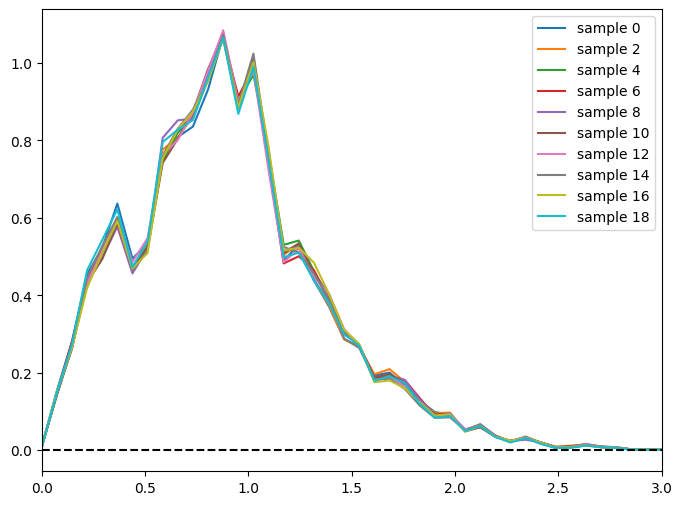
Naive stack just “stacks” i.e. sums up, the PDFs and returns a qp.interp distribution with bins defined by np.linspace(zmin, zmax, nzbins), we will create a stack with 41 bins and generate 20 bootstrap realizations

naive_results = ri.estimation.algos.naive_stack.naive_stack_summarizer(
    input_data=qp_data,
    zmin=0.0,
    zmax=3.0,
    nzbins=41,
    n_samples=20,
)

Inserting handle into data store.  input: None, NaiveStackSummarizer
Process 0 running estimator on chunk 0 - 20,449

Inserting handle into data store.  output: inprogress_output.hdf5, NaiveStackSummarizer
Inserting handle into data store.  single_NZ: inprogress_single_NZ.hdf5, NaiveStackSummarizer

The results are now in naive_results, but because of the DataStore, the actual ensemble is stored in .data, let’s grab the ensemble and plot a few of the bootstrap sample N(z) estimates:

newens = naive_results["output"]

fig, axs = plt.subplots(figsize=(8, 6))
for i in range(0, 20, 2):
    newens[i].plot_native(axes=axs, label=f"sample {i}")
axs.plot([0, 3], [0, 0], "k--")
axs.set_xlim(0, 3)
axs.legend(loc="upper right")

<matplotlib.legend.Legend at 0x7f3e748dd780>

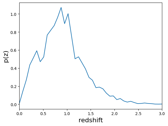
The summarizer also outputs a second file containing the fiducial N(z). We saved the fiducial N(z) in the file “NaiveStack_NZ.hdf5”, let’s grab the N(z) estimate with qp and plot it with the native plotter:

naive_nz = naive_results["single_NZ"]
naive_nz.plot_native(xlim=(0, 3))

<Axes: xlabel='redshift', ylabel='p(z)'>

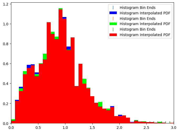
Point Estimate Hist

PointEstHistSummarizer takes the point estimate mode of each PDF and then histograms these, we’ll again generate 41 bootstrap samples of this and plot a few of the resultant histograms. Note: For some reason the plotting on the histogram distribution in qp is a little wonky, it appears alpha is broken, so this plot is not the best:

pens = ri.estimation.algos.point_est_hist.point_est_hist_summarizer(
    input_data=qp_data,
    zmin=0.0,
    zmax=3.0,
    nzbins=41,
    n_samples=20,
)["output"]

Inserting handle into data store.  input: None, PointEstHistSummarizer
Process 0 running estimator on chunk 0 - 20,449

Inserting handle into data store.  output: inprogress_output.hdf5, PointEstHistSummarizer
Inserting handle into data store.  single_NZ: inprogress_single_NZ.hdf5, PointEstHistSummarizer

fig, axs = plt.subplots(figsize=(8, 6))
pens[0].plot_native(axes=axs, fc=[0, 0, 1, 0.01])
pens[1].plot_native(axes=axs, fc=[0, 1, 0, 0.01])
pens[4].plot_native(axes=axs, fc=[1, 0, 0, 0.01])
axs.set_xlim(0, 3)
axs.legend()

<matplotlib.legend.Legend at 0x7f3ee104d390>

Again, we have saved the fiducial N(z) in a separate file, “point_NZ.hdf5”, we could read that data in if we desired.

VarInfStackSummarizer

VarInfStackSummarizer implements Markus’ variational inference scheme and returns qp.interp gridded distribution. VarInfStackSummarizer tends to get a little wonky if you use too many bins, so we’ll only use 25 bins. Again let’s generate 20 samples and plot a few:

vens = ri.estimation.algos.var_inf.var_inf_stack_summarizer(
    input_data=qp_data, zmin=0.0, zmax=3.0, nzbins=25, niter=10, n_samples=10
)
vens

Inserting handle into data store.  input: None, VarInfStackSummarizer
Process 0 running estimator on chunk 0 - 20,449

Inserting handle into data store.  output: inprogress_output.hdf5, VarInfStackSummarizer
Inserting handle into data store.  single_NZ: inprogress_single_NZ.hdf5, VarInfStackSummarizer

{'output': Ensemble(the_class=interp,shape=(10, 25)),
 'single_NZ': Ensemble(the_class=interp,shape=(1, 25))}

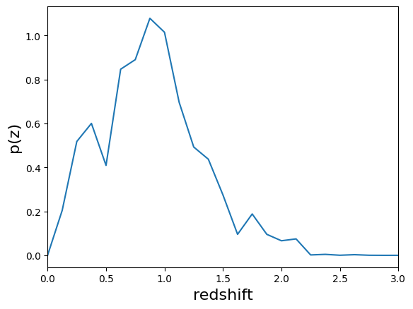
Let’s plot the fiducial N(z) for this distribution:

varinf_nz = vens["single_NZ"]
varinf_nz.plot_native(xlim=(0, 3))

<Axes: xlabel='redshift', ylabel='p(z)'>

NZDir

NZDirSummarizer is a different type of summarizer, taking a weighted set of neighbors to a set of training spectroscopic objects to reconstruct the redshift distribution of the photometric sample. I implemented a bootstrap of the spectroscopic data rather than the photometric data, both because it was much easier computationally, and I think that the spectroscopic variance is more important to take account of than simple bootstrap of the large photometric sample. We must first run the inform_NZDir stage to train up the K nearest neigh tree used by NZDirSummarizer, then we will run NZDirSummarizer to actually construct the N(z) estimate.

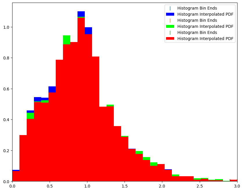
Like PointEstHistSummarizer NZDirSummarizer returns a qp.hist ensemble of samples

nzdir_model = ri.estimation.algos.nz_dir.nz_dir_informer(
    training_data=training_data, n_neigh=8
)["model"]

Inserting handle into data store.  input: None, NZDirInformer
Inserting handle into data store.  model: inprogress_model.pkl, NZDirInformer

nzd_summary = ri.estimation.algos.nz_dir.nz_dir_summarizer(
    input_data=test_data,
    leafsize=20,
    zmin=0.0,
    zmax=3.0,
    nzbins=31,
    model=nzdir_model,
    hdf5_groupname="photometry",
)

Inserting handle into data store.  input: None, NZDirSummarizer
Inserting handle into data store.  model: {'distances': array([3.93343151, 0.99550861, 0.502487  , ..., 0.55141209, 0.52943015,
       0.34063373], shape=(10225,)), 'szusecols': ['mag_u_lsst', 'mag_g_lsst', 'mag_r_lsst', 'mag_i_lsst', 'mag_z_lsst', 'mag_y_lsst'], 'szweights': array([1., 1., 1., ..., 1., 1., 1.], shape=(10225,)), 'szvec': array([0.02043499, 0.01936132, 0.03672067, ..., 2.97927326, 2.98694714,
       2.97646626], shape=(10225,)), 'sz_mag_data': array([[18.040369, 16.960892, 16.653412, 16.50631 , 16.466377, 16.423904],
       [21.61559 , 20.709402, 20.533852, 20.437565, 20.408886, 20.38821 ],
       [21.851952, 20.437067, 19.709715, 19.31263 , 18.953411, 18.770441],
       ...,
       [25.185795, 24.11405 , 23.828472, 23.711334, 23.75624 , 23.83491 ],
       [26.682219, 25.068745, 24.770744, 24.587885, 24.786388, 24.673431],
       [26.926563, 25.552408, 24.984402, 24.891462, 24.842054, 24.777039]],
      shape=(10225, 6), dtype=float32)}, NZDirSummarizer
Process 0 running estimator on chunk 0 - 20449

Inserting handle into data store.  single_NZ: inprogress_single_NZ.hdf5, NZDirSummarizer
Inserting handle into data store.  output: inprogress_output.hdf5, NZDirSummarizer

nzd_ens = nzd_summary["output"]
nzdir_nz = nzd_summary["single_NZ"]

fig, axs = plt.subplots(figsize=(10, 8))
nzd_ens[0].plot_native(axes=axs, fc=[0, 0, 1, 0.01])
nzd_ens[1].plot_native(axes=axs, fc=[0, 1, 0, 0.01])
nzd_ens[4].plot_native(axes=axs, fc=[1, 0, 0, 0.01])
axs.set_xlim(0, 3)
axs.legend()

<matplotlib.legend.Legend at 0x7f3ec7fd7760>

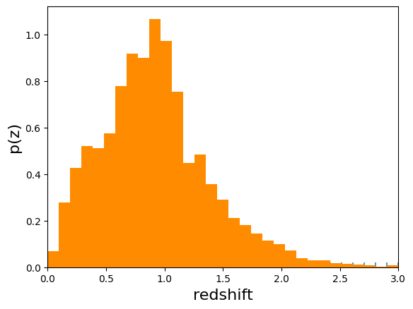
As we also wrote out the single estimate of N(z) we can read that data from the second file written (specified by the single_NZ argument given in NZDirSummarizer.make_stage above, in this case “NZDir_NZ.hdf5”)

nzdir_nz.plot_native(xlim=(0, 3))

<Axes: xlabel='redshift', ylabel='p(z)'>

Results

All three results files are qp distributions, NaiveStackSummarizer and VarInfStackSummarizer return qp.interp distributions while PointEstHistSummarizer returns a qp.histogram distribution. Even with the different distributions you can use qp functionality to do things like determine the means, modes, etc… of the distributions. You could then use the std dev of any of these to estimate a 1 sigma “shift”, etc…

zgrid = np.linspace(0, 3, 41)
names = ["naive", "point", "varinf", "nzdir"]
enslist = [newens, pens, vens["output"], nzd_ens]
results_dict = {}
for nm, en in zip(names, enslist):
    results_dict[f"{nm}_modes"] = en.mode(grid=zgrid).flatten()
    results_dict[f"{nm}_means"] = en.mean().flatten()
    results_dict[f"{nm}_std"] = en.std().flatten()

results_dict

{'naive_modes': array([0.9, 0.9, 0.9, 0.9, 0.9, 0.9, 0.9, 0.9, 0.9, 0.9, 0.9, 0.9, 0.9,
        0.9, 0.9, 0.9, 0.9, 0.9, 0.9, 0.9]),
 'naive_means': array([0.90186015, 0.90594959, 0.90998413, 0.90789723, 0.91061713,
        0.91218896, 0.90767783, 0.90533378, 0.90791096, 0.90745548,
        0.91191782, 0.90432094, 0.90620407, 0.9087479 , 0.90410093,
        0.91160362, 0.90904143, 0.90900628, 0.89714565, 0.9139707 ]),
 'naive_std': array([0.45914047, 0.45888175, 0.45996851, 0.45790462, 0.45714307,
        0.46346092, 0.45902071, 0.45676502, 0.45571704, 0.45996679,
        0.45816316, 0.4557761 , 0.45894757, 0.45615512, 0.45516466,
        0.45840581, 0.4548986 , 0.4602565 , 0.45546553, 0.45910612]),
 'point_modes': array([0.9, 0.9, 0.9, 0.9, 0.9, 0.9, 0.9, 0.9, 0.9, 0.9, 0.9, 0.9, 0.9,
        0.9, 0.9, 0.9, 0.9, 0.9, 0.9, 0.9]),
 'point_means': array([0.89950191, 0.90316242, 0.90687302, 0.90601783, 0.90864065,
        0.90872653, 0.90396036, 0.90296562, 0.90483344, 0.90456865,
        0.90957456, 0.90098687, 0.9043146 , 0.90417863, 0.90164168,
        0.90770316, 0.90771032, 0.90617885, 0.89527605, 0.90990018]),
 'point_std': array([0.451436  , 0.4514502 , 0.45148951, 0.45006287, 0.45043543,
        0.45565337, 0.44891521, 0.4484236 , 0.44829022, 0.4508991 ,
        0.4500663 , 0.4485642 , 0.45077344, 0.44607659, 0.44649072,
        0.44982927, 0.44799803, 0.45198245, 0.44738948, 0.44999159]),
 'varinf_modes': array([0.9  , 0.9  , 0.9  , 0.9  , 0.975, 0.9  , 0.9  , 0.9  , 0.9  ,
        0.9  ]),
 'varinf_means': array([0.89003845, 0.89392636, 0.89344345, 0.89527312, 0.89632345,
        0.89302009, 0.89468313, 0.89474443, 0.88888415, 0.89065952]),
 'varinf_std': array([0.42668055, 0.43098261, 0.42998022, 0.42472522, 0.42612753,
        0.4260668 , 0.4298318 , 0.42863912, 0.42913894, 0.42877965]),
 'nzdir_modes': array([0.9, 0.9, 0.9, 0.9, 0.9, 0.9, 0.9, 0.9, 0.9, 0.9, 0.9, 0.9, 0.9,
        0.9, 0.9, 0.9, 0.9, 0.9, 0.9, 0.9]),
 'nzdir_means': array([0.91527627, 0.92144451, 0.92166271, 0.92410584, 0.92118734,
        0.91847357, 0.92651638, 0.91452663, 0.92038542, 0.92942564,
        0.93107928, 0.91022267, 0.92142493, 0.92510869, 0.91931933,
        0.92364447, 0.919305  , 0.92659316, 0.91014124, 0.92499533]),
 'nzdir_std': array([0.46761557, 0.47080438, 0.46766624, 0.46515462, 0.46097655,
        0.46587178, 0.46626591, 0.46660589, 0.4646169 , 0.47014536,
        0.47077795, 0.46410977, 0.46431021, 0.46323947, 0.46435023,
        0.47121424, 0.46146407, 0.46880833, 0.46674124, 0.46798514])}

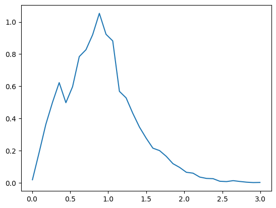
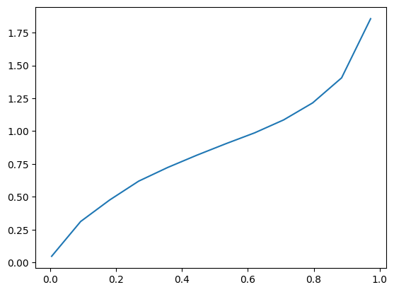
You can also use qp to compute quantities the pdf, cdf, ppf, etc… on any grid that you want, much of the functionality of scipy.stats distributions have been inherited by qp ensembles

newgrid = np.linspace(0.005, 2.995, 35)
naive_pdf = newens.pdf(newgrid)
point_cdf = pens.cdf(newgrid)
var_ppf = vens["output"].ppf(newgrid)

plt.plot(newgrid, naive_pdf[0])

[<matplotlib.lines.Line2D at 0x7f3ec780b7f0>]

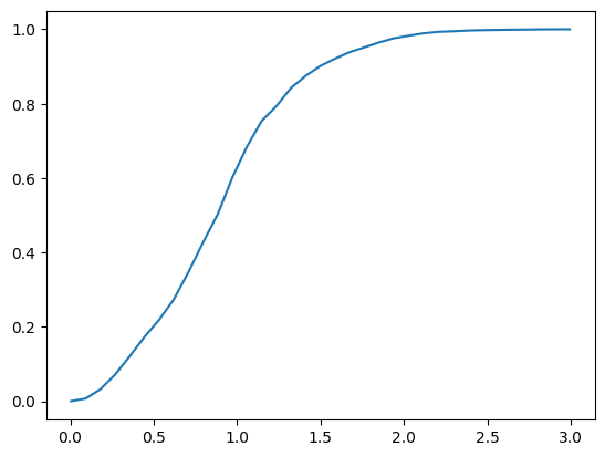
plt.plot(newgrid, point_cdf[0])

[<matplotlib.lines.Line2D at 0x7f3ec7a34400>]

plt.plot(newgrid, var_ppf[0])

[<matplotlib.lines.Line2D at 0x7f3ec7a6c3d0>]

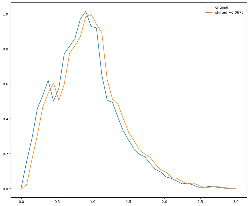
Shifts

If you want to “shift” a PDF, you can just evaluate the PDF on a shifted grid, for example to shift the PDF by +0.0375 in redshift you could evaluate on a shifted grid. For now we can just do this “by hand”, we could easily implement shift functionality in qp, I think.

def_grid = np.linspace(0.0, 3.0, 41)
shift_grid = def_grid - 0.0675
native_nz = newens.pdf(def_grid)
shift_nz = newens.pdf(shift_grid)

fig = plt.figure(figsize=(12, 10))
plt.plot(def_grid, native_nz[0], label="original")
plt.plot(def_grid, shift_nz[0], label="shifted +0.0675")
plt.legend(loc="upper right")

<matplotlib.legend.Legend at 0x7f3ec7c4ed70>

You can estimate how much shift you might expect based on the statistics of our bootstrap samples, say the std dev of the means for the NZDir-derived distribution:

results_dict["nzdir_means"]

array([0.91527627, 0.92144451, 0.92166271, 0.92410584, 0.92118734,
       0.91847357, 0.92651638, 0.91452663, 0.92038542, 0.92942564,
       0.93107928, 0.91022267, 0.92142493, 0.92510869, 0.91931933,
       0.92364447, 0.919305  , 0.92659316, 0.91014124, 0.92499533])

spread = np.std(results_dict["nzdir_means"])

spread

np.float64(0.005498408843907313)

Again, not a huge spread in predicted mean redshifts based solely on bootstraps, even with only ~20,000 galaxies.