RAIL Estimation Tutorial Notebook

Authors: Sam Schmidt, Eric Charles, Alex Malz, others…

Last run successfully: August 15, 2023

This is a notebook demonstrating some of the estimation features of the LSST-DESC RAIL-iverse packages.

The rail.estimation subpackage contains infrastructure to run multiple production-level photo-z codes. There is a minimimal superclass that sets up some file paths and variable names. Each specific photo-z code resides in a subclass in rail.estimation.algos with algorithm-specific setup variables. More extensive documentation is available on Read the Docs here: https://rail-hub.readthedocs.io/en/latest/

Note: If you’re planning to run this in a notebook, you may want to use interactive mode instead. See Quick_Start_in_Estimation.ipynb in the interactive_examples/estimation_examples/ folder for a version of this notebook in interactive mode.

import os
import matplotlib.pyplot as plt
import numpy as np
%matplotlib inline

import rail
import qp
import tables_io
from rail.core.data import TableHandle
from rail.core.stage import RailStage

Importing all available estimators

There is some handy functionality in rail.stages to import all available stages that are installed in your environment. RailStage knows about all of the sub-types of stages. By looping through the values in the RailStage.pipeline_stages dictionary, we can isolate those that are sub-classes of rail.estimation.estimator.CatEstimator, which operate on catalog-like inputs. Let’s run this import_and_attach_all() command, and then print out the subclasses that are now available for use (though in this demo we only take advantage of two specific estimators):

import rail.stages
rail.stages.import_and_attach_all()

for val in RailStage.pipeline_stages.values():
    if issubclass(val[0], rail.estimation.estimator.CatEstimator):
        print(val[0])

Imported rail.astro_tools
Imported rail.bpz
Imported rail.cmnn
Imported rail.core

Imported rail.dnf

Imported rail.dsps
Imported rail.flexzboost

Install FSPS with the following commands:
pip uninstall fsps
git clone --recursive https://github.com/dfm/python-fsps.git
cd python-fsps
python -m pip install .
export SPS_HOME=$(pwd)/src/fsps/libfsps

Imported rail.fsps
Imported rail.gpz
Imported rail.hub
LEPHAREDIR is being set to the default cache directory:
/home/runner/.cache/lephare/data
More than 1Gb may be written there.
LEPHAREWORK is being set to the default cache directory:
/home/runner/.cache/lephare/work
Default work cache is already linked.
This is linked to the run directory:
/home/runner/.cache/lephare/runs/20260601T150817

A module that was compiled using NumPy 1.x cannot be run in
NumPy 2.2.6 as it may crash. To support both 1.x and 2.x
versions of NumPy, modules must be compiled with NumPy 2.0.
Some module may need to rebuild instead e.g. with 'pybind11>=2.12'.

If you are a user of the module, the easiest solution will be to
downgrade to 'numpy<2' or try to upgrade the affected module.
We expect that some modules will need time to support NumPy 2.

Traceback (most recent call last):  File "/opt/hostedtoolcache/Python/3.10.20/x64/lib/python3.10/runpy.py", line 196, in _run_module_as_main
    return _run_code(code, main_globals, None,
  File "/opt/hostedtoolcache/Python/3.10.20/x64/lib/python3.10/runpy.py", line 86, in _run_code
    exec(code, run_globals)
  File "/opt/hostedtoolcache/Python/3.10.20/x64/lib/python3.10/site-packages/ipykernel_launcher.py", line 18, in <module>
    app.launch_new_instance()
  File "/opt/hostedtoolcache/Python/3.10.20/x64/lib/python3.10/site-packages/traitlets/config/application.py", line 1082, in launch_instance
    app.start()
  File "/opt/hostedtoolcache/Python/3.10.20/x64/lib/python3.10/site-packages/ipykernel/kernelapp.py", line 758, in start
    self.io_loop.start()
  File "/opt/hostedtoolcache/Python/3.10.20/x64/lib/python3.10/site-packages/tornado/platform/asyncio.py", line 211, in start
    self.asyncio_loop.run_forever()
  File "/opt/hostedtoolcache/Python/3.10.20/x64/lib/python3.10/asyncio/base_events.py", line 603, in run_forever
    self._run_once()
  File "/opt/hostedtoolcache/Python/3.10.20/x64/lib/python3.10/asyncio/base_events.py", line 1909, in _run_once
    handle._run()
  File "/opt/hostedtoolcache/Python/3.10.20/x64/lib/python3.10/asyncio/events.py", line 80, in _run
    self._context.run(self._callback, *self._args)
  File "/opt/hostedtoolcache/Python/3.10.20/x64/lib/python3.10/site-packages/ipykernel/utils.py", line 71, in preserve_context
    return await f(*args, **kwargs)
  File "/opt/hostedtoolcache/Python/3.10.20/x64/lib/python3.10/site-packages/ipykernel/kernelbase.py", line 621, in shell_main
    await self.dispatch_shell(msg, subshell_id=subshell_id)
  File "/opt/hostedtoolcache/Python/3.10.20/x64/lib/python3.10/site-packages/ipykernel/kernelbase.py", line 478, in dispatch_shell
    await result
  File "/opt/hostedtoolcache/Python/3.10.20/x64/lib/python3.10/site-packages/ipykernel/ipkernel.py", line 372, in execute_request
    await super().execute_request(stream, ident, parent)
  File "/opt/hostedtoolcache/Python/3.10.20/x64/lib/python3.10/site-packages/ipykernel/kernelbase.py", line 834, in execute_request
    reply_content = await reply_content
  File "/opt/hostedtoolcache/Python/3.10.20/x64/lib/python3.10/site-packages/ipykernel/ipkernel.py", line 464, in do_execute
    res = shell.run_cell(
  File "/opt/hostedtoolcache/Python/3.10.20/x64/lib/python3.10/site-packages/ipykernel/zmqshell.py", line 663, in run_cell
    return super().run_cell(*args, **kwargs)
  File "/opt/hostedtoolcache/Python/3.10.20/x64/lib/python3.10/site-packages/IPython/core/interactiveshell.py", line 3077, in run_cell
    result = self._run_cell(
  File "/opt/hostedtoolcache/Python/3.10.20/x64/lib/python3.10/site-packages/IPython/core/interactiveshell.py", line 3132, in _run_cell
    result = runner(coro)
  File "/opt/hostedtoolcache/Python/3.10.20/x64/lib/python3.10/site-packages/IPython/core/async_helpers.py", line 128, in _pseudo_sync_runner
    coro.send(None)
  File "/opt/hostedtoolcache/Python/3.10.20/x64/lib/python3.10/site-packages/IPython/core/interactiveshell.py", line 3336, in run_cell_async
    has_raised = await self.run_ast_nodes(code_ast.body, cell_name,
  File "/opt/hostedtoolcache/Python/3.10.20/x64/lib/python3.10/site-packages/IPython/core/interactiveshell.py", line 3519, in run_ast_nodes
    if await self.run_code(code, result, async_=asy):
  File "/opt/hostedtoolcache/Python/3.10.20/x64/lib/python3.10/site-packages/IPython/core/interactiveshell.py", line 3579, in run_code
    exec(code_obj, self.user_global_ns, self.user_ns)
  File "/tmp/ipykernel_7187/4014131292.py", line 2, in <module>
    rail.stages.import_and_attach_all()
  File "/opt/hostedtoolcache/Python/3.10.20/x64/lib/python3.10/site-packages/rail/stages/__init__.py", line 74, in import_and_attach_all
    RailEnv.import_all_packages(silent=silent)
  File "/opt/hostedtoolcache/Python/3.10.20/x64/lib/python3.10/site-packages/rail/core/introspection.py", line 541, in import_all_packages
    _imported_module = importlib.import_module(pkg)
  File "/opt/hostedtoolcache/Python/3.10.20/x64/lib/python3.10/importlib/__init__.py", line 126, in import_module
    return _bootstrap._gcd_import(name[level:], package, level)
  File "/opt/hostedtoolcache/Python/3.10.20/x64/lib/python3.10/site-packages/rail/interactive/__init__.py", line 3, in <module>
    from . import calib, creation, estimation, evaluation, tools
  File "/opt/hostedtoolcache/Python/3.10.20/x64/lib/python3.10/site-packages/rail/interactive/calib/__init__.py", line 3, in <module>
    from rail.utils.interactive.initialize_utils import _initialize_interactive_module
  File "/opt/hostedtoolcache/Python/3.10.20/x64/lib/python3.10/site-packages/rail/utils/interactive/initialize_utils.py", line 17, in <module>
    from rail.utils.interactive.base_utils import (
  File "/opt/hostedtoolcache/Python/3.10.20/x64/lib/python3.10/site-packages/rail/utils/interactive/base_utils.py", line 10, in <module>
    rail.stages.import_and_attach_all(silent=True)
  File "/opt/hostedtoolcache/Python/3.10.20/x64/lib/python3.10/site-packages/rail/stages/__init__.py", line 74, in import_and_attach_all
    RailEnv.import_all_packages(silent=silent)
  File "/opt/hostedtoolcache/Python/3.10.20/x64/lib/python3.10/site-packages/rail/core/introspection.py", line 541, in import_all_packages
    _imported_module = importlib.import_module(pkg)
  File "/opt/hostedtoolcache/Python/3.10.20/x64/lib/python3.10/importlib/__init__.py", line 126, in import_module
    return _bootstrap._gcd_import(name[level:], package, level)
  File "/opt/hostedtoolcache/Python/3.10.20/x64/lib/python3.10/site-packages/rail/som/__init__.py", line 1, in <module>
    from rail.creation.degraders.specz_som import *
  File "/opt/hostedtoolcache/Python/3.10.20/x64/lib/python3.10/site-packages/rail/creation/degraders/specz_som.py", line 15, in <module>
    from somoclu import Somoclu
  File "/opt/hostedtoolcache/Python/3.10.20/x64/lib/python3.10/site-packages/somoclu/__init__.py", line 11, in <module>
    from .train import Somoclu
  File "/opt/hostedtoolcache/Python/3.10.20/x64/lib/python3.10/site-packages/somoclu/train.py", line 25, in <module>
    from .somoclu_wrap import train as wrap_train
  File "/opt/hostedtoolcache/Python/3.10.20/x64/lib/python3.10/site-packages/somoclu/somoclu_wrap.py", line 11, in <module>
    import _somoclu_wrap

---------------------------------------------------------------------------

ImportError                               Traceback (most recent call last)

File /opt/hostedtoolcache/Python/3.10.20/x64/lib/python3.10/site-packages/numpy/core/_multiarray_umath.py:44, in __getattr__(attr_name)
     39     # Also print the message (with traceback).  This is because old versions
     40     # of NumPy unfortunately set up the import to replace (and hide) the
     41     # error.  The traceback shouldn't be needed, but e.g. pytest plugins
     42     # seem to swallow it and we should be failing anyway...
     43     sys.stderr.write(msg + tb_msg)
---> 44     raise ImportError(msg)
     46 ret = getattr(_multiarray_umath, attr_name, None)
     47 if ret is None:


ImportError:
A module that was compiled using NumPy 1.x cannot be run in
NumPy 2.2.6 as it may crash. To support both 1.x and 2.x
versions of NumPy, modules must be compiled with NumPy 2.0.
Some module may need to rebuild instead e.g. with 'pybind11>=2.12'.

If you are a user of the module, the easiest solution will be to
downgrade to 'numpy<2' or try to upgrade the affected module.
We expect that some modules will need time to support NumPy 2.

Warning: the binary library cannot be imported. You cannot train maps, but you can load and analyze ones that you have already saved.
The problem occurs because either compilation failed when you installed Somoclu or a path is missing from the dependencies when you are trying to import it. Please refer to the documentation to see your options.

Imported rail.interactive
Imported rail.interfaces
Imported rail.lephare
Imported rail.pzflow
Imported rail.sklearn
Imported rail.som
Imported rail.stages
Imported rail.yaw_rail
Attached 16 base classes and 98 fully formed stages to rail.stages
<class 'rail.estimation.estimator.CatEstimator'>
<class 'rail.estimation.algos.random_gauss.RandomGaussEstimator'>
<class 'rail.estimation.algos.train_z.TrainZEstimator'>
<class 'rail.estimation.algos.bpz_lite.BPZliteEstimator'>
<class 'rail.estimation.algos.cmnn.CMNNEstimator'>
<class 'rail.estimation.algos.dnf.DNFEstimator'>
<class 'rail.estimation.algos.flexzboost.FlexZBoostEstimator'>
<class 'rail.estimation.algos.gpz.GPzEstimator'>
<class 'rail.estimation.algos.lephare.LephareEstimator'>
<class 'rail.estimation.algos.pzflow_nf.PZFlowEstimator'>
<class 'rail.estimation.algos.k_nearneigh.KNearNeighEstimator'>
<class 'rail.estimation.algos.nz_dir.NZDirSummarizer'>
<class 'rail.estimation.algos.sklearn_neurnet.SklNeurNetEstimator'>

You should see a list of the available subclasses corresponding to specific photo-z algorithms, as printed out above. These currently include:

bpz_lite is a template-based code that outputs the posterior estimated given a specific template set and Bayesian prior. See Benitez (2000) for more details.
cmnn is an implementation of the “colour-matched nearest neighbour` estimator described in Graham et al 2018. It returns a single Gaussian for each galaxy.
delight_hybrid (currently delightPZ) is a hybrid gaussian process/template-based code. See the Leistedt & Hogg (2017) for more details.
flexzboost is a fully functional photo-z algorithm, implementing the FlexZBoost conditional density estimate method from Izbicki, Lee & Freeman (2017) that performed well in the LSST-DESC Photo-Z Data Challenge 1 paper (Schmidt, Malz & Soo, et al. (2020)). FlexZBoost and some specialized metrics for it are available in Python and R through FlexCode.
gpz is a Gaussian Process-based estimator. See Almosallam et al 2016 for details on the algorithm. It currently returns a single Gaussian for each PDF.
k_nearneigh is a simple implementation of a weighted k-nearest neighbor photo-z code. It stores each PDF as a weighted sum of Gaussians based on the distance from neighbors in color-space.
pzflow_nf uses the same normalizing flow code pzflow, the same one that appears in rail.creation, to predict redshift PDFs.
random_gauss is a very simple class that does not actually predict a meaningful photo-z but can be useful for quick null tests when developing a pipeline. Instead it produces a randomly drawn Gaussian for each galaxy.
sklearn_neurnet is another toy model using sklearn’s neural network to predict a point estimate redshift from the training data, then assigns a sigma width based on the estimated redshift.
trainz is our “pathological” estimator. It makes a PDF from a histogram of the training data and assigns that PDF to every galaxy without considering its photometry.

Each code should have two specific classes associated with it: one to inform() using a set of training data or explicit priors and one to estimate() the per-galaxy photo-z PDFs. These should be imported from the src/rail/estimation/algos/[name_of_code] module using the above names. The naming pattern is [NameOfCode]Estimator for the estimating class, and [NameOfCode]Informer for the training/ingesting class, for example FlexZBoostEstimator and FlexZBoostInformer.

For each of these two classes, we follow the pattern to first run a make_stage() method for the class in order to set up the ceci infrastructure and then invoke the inform() or estimate() method for the class in question. We show examples of this below.

The code-specific parameters

Each photo-z algorithm has code-specific parameters necessary to initialize the code. These values can be input on the command line, or passed in via a dictionary.

Let’s start with a very simple demonstration using k_nearneigh, a RAIL wrapper around sklearn’s nearest neighbor (NN) method. It calculates a normalized weight for the K nearest neighbors based on their distance and makes a PDF as a sum of K Gaussians, each at the redshift of the training galaxy with amplitude based on the distance weight, and a Gaussian width set by the user. This is a toy model estimator, but it actually performs very well for representative data sets. There are configuration parameters for the names of columns, random seeds, etc… in KNearNeighEstimator with best-guess sensible defaults based on preliminary experimentation in DESC. See the KNearNeigh code for more details, but here is a minimal set to run:

knn_dict = dict(zmin=0.0, zmax=3.0, nzbins=301, trainfrac=0.75,
                sigma_grid_min=0.01, sigma_grid_max=0.07, ngrid_sigma=10,
                nneigh_min=3, nneigh_max=7, hdf5_groupname='photometry')

Here, trainfrac sets the proportion of training data to use in training the algorithm, where the remaining fraction is used to validate both the width of the Gaussians used in constructing the PDF and the number of neighbors used in each PDF. The CDE Loss is a metric computed on a grid of some width and number of neighbors, and the combination of width and number of neighbors with the lowest CDE loss is used. sigma_grid_min, sigma_grid_max, and ngrid_sigma are used to specify the grid of sigma values to test, while nneigh_min and nneigh_max are the integer values between which we will check the loss.

zmin, zmax, and nzbins are used to create a grid on which the CDE Loss is computed when minimizing the loss to find the best values for sigma and number of neighbors to use.

We will begin by training the algorithm by instantiating its Informer stage.

If any essential parameters are missing from the parameter dictionary, they will be set to default values:

from rail.estimation.algos.k_nearneigh import KNearNeighInformer, KNearNeighEstimator
pz_train = KNearNeighInformer.make_stage(name='inform_KNN', model='demo_knn.pkl', **knn_dict)

Now, let’s load our training data, which is stored in hdf5 format. We’ll load it into the DataStore so that the ceci stages are able to access it.

from rail.utils.path_utils import find_rail_file
trainFile = find_rail_file('examples_data/testdata/test_dc2_training_9816.hdf5')
testFile = find_rail_file('examples_data/testdata/test_dc2_validation_9816.hdf5')
training_data=tables_io.read(trainFile)
test_data=tables_io.read(testFile)
# training_data = DS.read_file("training_data", TableHandle, trainFile)
# test_data = DS.read_file("test_data", TableHandle, testFile)

We need to train the KDTree, which is done with the inform() method present in every Informer stage. The parameter model is the name that the trained model object that will be saved as, in a format specific to the estimation algorithm in question. In this case the format is a pickle file called demo_knn.pkl.

KNearNeighInformer.inform finds the best sigma and NNeigh and stores those along with the KDTree in the model.

%%time
pz_train.inform(training_data)

Inserting handle into data store.  input: None, inform_KNN
split into 7669 training and 2556 validation samples
finding best fit sigma and NNeigh...

best fit values are sigma=0.023333333333333334 and numneigh=7

Inserting handle into data store.  model_inform_KNN: inprogress_demo_knn.pkl, inform_KNN
CPU times: user 8.83 s, sys: 1.5 s, total: 10.3 s
Wall time: 10.3 s

<rail.core.data.ModelHandle at 0x7fd250a2b700>

We can now set up the main photo-z Estimator stage and run our algorithm on the data to produce simple photo-z estimates. Note that we are loading the trained model that we computed from the Informer stage:

pz = KNearNeighEstimator.make_stage(name='KNN', hdf5_groupname='photometry',
                              model=pz_train.get_handle('model'))
results = pz.estimate(test_data)

Inserting handle into data store.  input: None, KNN
Inserting handle into data store.  model_inform_KNN: <class 'rail.core.data.ModelHandle'> demo_knn.pkl, (wd), KNN
Process 0 running estimator on chunk 0 - 20,449
Process 0 estimating PZ PDF for rows 0 - 20,449

Inserting handle into data store.  output_KNN: inprogress_output_KNN.hdf5, KNN

The output file is a qp.Ensemble containing the redshift PDFs. This Ensemble also includes a photo-z point estimate derived from the PDFs, the mode by default (though there will soon be a keyword option to choose a different point estimation method or to skip the calculation of a point estimate). The modes are stored in the “ancillary” data within the Ensemble. By default it will be in an 1xM array, so you may need to include a .flatten() to flatten the array. The zmode values in the ancillary data can be accessed via:

zmode = results().ancil['zmode'].flatten()

Let’s plot the redshift mode against the true redshifts to see how they look:

plt.figure(figsize=(8,8))
plt.scatter(test_data['photometry']['redshift'],zmode,s=1,c='k',label='simple NN mode')
plt.plot([0,3],[0,3],'r--')
plt.xlabel("true redshift")
plt.ylabel("simple NN photo-z")

Text(0, 0.5, 'simple NN photo-z')

../../../_images/00_Quick_Start_in_Estimation_21_1.png

Not bad, given our very simple estimator! For the PDFs, KNearNeigh is storing each PDF as a Gaussian mixture model parameterization where each PDF is represented by a set of N Gaussians for each galaxy. qp.Ensemble objects have all the methods of scipy.stats.rv_continuous objects so we can evaluate the PDF on a set of grid points with the built-in .pdf method. Let’s pick a single galaxy from our sample and evaluate and plot the PDF, the mode, and true redshift:

zgrid = np.linspace(0, 3., 301)

galid = 9529
single_gal = np.squeeze(results()[galid].pdf(zgrid))
single_zmode = zmode[galid]
truez = test_data['photometry']['redshift'][galid]
plt.plot(zgrid,single_gal,color='k',label='single pdf')
plt.axvline(single_zmode,color='k', ls='--', label='mode')
plt.axvline(truez,color='r',label='true redshift')
plt.legend(loc='upper right')
plt.xlabel("redshift")
plt.ylabel("p(z)")

Text(0, 0.5, 'p(z)')

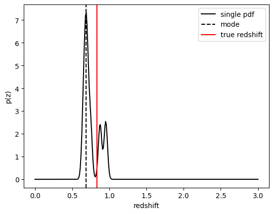
../../../_images/00_Quick_Start_in_Estimation_24_1.png

We see that KNearNeigh PDFs do consist of a number of discrete Gaussians, and many have quite a bit of substructure. This is a naive estimator, and some of these features are likely spurious.

FlexZBoost

That illustrates the basics. Now let’s try the FlexZBoostEstimator estimator. FlexZBoost is available in the rail_flexzboost repo and can be installed with

pip install pz-rail-flexzboost

on the command line or from source. Once installed, it will function the same as any of the other estimators included in the primary rail repo.

FlexZBoostEstimator approximates the conditional density estimate for each PDF with a set of weights on a set of basis functions. This can save space relative to a gridded parameterization, but it also leads to residual “bumps” in the PDF intrinsic to the underlying cosine or fourier parameterization. For this reason, FlexZBoostEstimator has a post-processing stage where it “trims” (i.e. sets to zero) any small peaks, or “bumps”, below a certain bump_thresh threshold.

One of the dominant features seen in our PhotoZDC1 analysis of multiple photo-z codes (Schmidt, Malz et al. 2020) was that photo-z estimates were often, in general, overconfident or underconfident in their overall uncertainty in PDFs. To remedy this, FlexZBoostEstimator has an additional post-processing step where it applies a “sharpening” parameter sharpen that modulates the width of the PDFs according to a power law.

A portion of the training data is held in reserve to determine best-fit values for both bump_thresh and sharpening, which we currently find by simply calculating the CDE loss for a grid of bump_thresh and sharpening values; once those values are set FlexZBoost will re-train its density estimate model with the full dataset. A more sophisticated hyperparameter fitting procedure may be implemented in the future.

We’ll start with a dictionary of setup parameters for FlexZBoostEstimator, just as we had for the k-nearest neighbor estimator. Some of the parameters are the same as in k-nearest neighbor above, zmin, zmax, nzbins. However, FlexZBoostEstimator performs a more in depth training and as such has more input parameters to control its behavior. These parameters are:

basis_system: which basis system to use in the density estimate. The default is cosine but fourier is also an option
max_basis: the maximum number of basis functions parameters to use for PDFs
regression_params: a dictionary of options fed to xgboost that control the maximum depth and the objective function. An update in xgboost means that objective should now be set to reg:squarederror for proper functioning.
trainfrac: The fraction of the training data to use for training the density estimate. The remaining galaxies will be used for validation of bump_thresh and sharpening.
bumpmin: the minimum value to test in the bump_thresh grid
bumpmax: the maximum value to test in the bump_thresh grid
nbump: how many points to test in the bump_thresh grid
sharpmin, sharpmax, nsharp: same as equivalent bump_thresh params, but for sharpening parameter

fz_dict = dict(zmin=0.0, zmax=3.0, nzbins=301,
               trainfrac=0.75, bumpmin=0.02, bumpmax=0.35,
               nbump=20, sharpmin=0.7, sharpmax=2.1, nsharp=15,
               max_basis=35, basis_system='cosine',
               hdf5_groupname='photometry',
               regression_params={'max_depth': 8,'objective':'reg:squarederror'})
fz_modelfile = 'demo_FZB_model.pkl'

from rail.estimation.algos.flexzboost import FlexZBoostInformer, FlexZBoostEstimator
inform_pzflex = FlexZBoostInformer.make_stage(name='inform_fzboost', model=fz_modelfile, **fz_dict)

FlexZBoostInformer operates on the training set and writes a file containing the estimation model. FlexZBoost uses xgboost to determine a conditional density estimate model, and also fits the bump_thresh and sharpen parameters described above.

FlexZBoost is a bit more sophisticated than the earlier k-nearest neighbor estimator, so it will take a bit longer to train, but not drastically so, still under a minute on a semi-new laptop. We specified the name of the model file, demo_FZB_model.pkl, which will store our trained model for use with the estimation stage.

%%time
inform_pzflex.inform(training_data)

Inserting handle into data store.  input: None, inform_fzboost
stacking some data...
read in training data
fit the model...

finding best bump thresh...

finding best sharpen parameter...

Retraining with full training set...

Best bump = 0.08947368421052632, best sharpen = 1.2
Inserting handle into data store.  model_inform_fzboost: inprogress_demo_FZB_model.pkl, inform_fzboost
CPU times: user 57.3 s, sys: 527 ms, total: 57.8 s
Wall time: 1min 1s

<rail.core.data.ModelHandle at 0x7fd235d43f10>

Loading a pre-trained model

If we have an existing pretrained model, for example the one in the file demo_FZB_model.pkl, we can skip this step in subsequent runs of an estimator; that is, we load this pickled model without having to repeat the training stage for this specific training data, and that can save time for larger training sets that would take longer to create the model.

There are two supported model output representations, interp (default) and flexzboost. Using flexzboost will store the output basis function weights from FlexCode, resulting in a smaller storage size on disk and giving the user the option to tune the sharpening and bump-removal parameters as a post-processing step. However, if you know that you will be performing operations on PDFs evaluated on a redshift grid that is known before performing the estimation, you can peform that post-processing up front by employing interp to store the output as interpolated y values for a given set of x values, requiring more storage space but eliminating the need to evaluate the PDFs upon downstream usage.

For additional comparisons of the approaches, see the documentation for qp_flexzboost here: https://qp-flexzboost.readthedocs.io/en/latest/source/performance_comparison.html

%%time
pzflex = FlexZBoostEstimator.make_stage(name='fzboost', hdf5_groupname='photometry',
                            model=inform_pzflex.get_handle('model'))

# For this notebook, we will use the default value of qp_representation as shown
# above due to the additional computation time that would be required in the
# later steps when working with the flexzboost representation.
# Below are two examples showing the explicit use of the qp_representation argument.
"""
pzflex = FlexZBoostEstimator.make_stage(name='fzboost', hdf5_groupname='photometry',
                            model=inform_pzflex.get_handle('model'),
                            qp_representation='interp')

pzflex = FlexZBoostEstimator.make_stage(name='fzboost', hdf5_groupname='photometry',
                            model=inform_pzflex.get_handle('model'),
                            qp_representation='flexzboost')
"""

CPU times: user 167 μs, sys: 7 μs, total: 174 μs
Wall time: 177 μs

"npzflex = FlexZBoostEstimator.make_stage(name='fzboost', hdf5_groupname='photometry',n                            model=inform_pzflex.get_handle('model'),n                            qp_representation='interp')nnpzflex = FlexZBoostEstimator.make_stage(name='fzboost', hdf5_groupname='photometry',n                            model=inform_pzflex.get_handle('model'),n                            qp_representation='flexzboost')n"

It takes only a few seconds, so, if you are running an algorithm with a burdensome training requirement, saving a trained copy of the model for later repeated use can be a real time saver.

Now, let’s compute photo-z’s using with the estimate method.

%%time
fzresults = pzflex.estimate(test_data)

Inserting handle into data store.  input: None, fzboost
Inserting handle into data store.  model_inform_fzboost: <class 'rail.core.data.ModelHandle'> demo_FZB_model.pkl, (wd), fzboost
Process 0 running estimator on chunk 0 - 20,449
Process 0 estimating PZ PDF for rows 0 - 20,449

Inserting handle into data store.  output_fzboost: inprogress_output_fzboost.hdf5, fzboost

CPU times: user 11.2 s, sys: 113 ms, total: 11.3 s
Wall time: 11.4 s

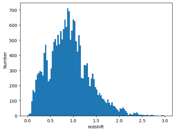
We can calculate the median and mode values of the PDFs and plot their distribution (in this case the modes are already stored in the qp.Ensemble’s ancillary data, but here is an example of computing the point estimates via qp directly):

fz_medians = fzresults().median()
fz_modes = fzresults().mode(grid=zgrid)

plt.hist(fz_medians, bins=np.linspace(-.005,3.005,101));
plt.xlabel("redshift")
plt.ylabel("Number")

Text(0, 0.5, 'Number')

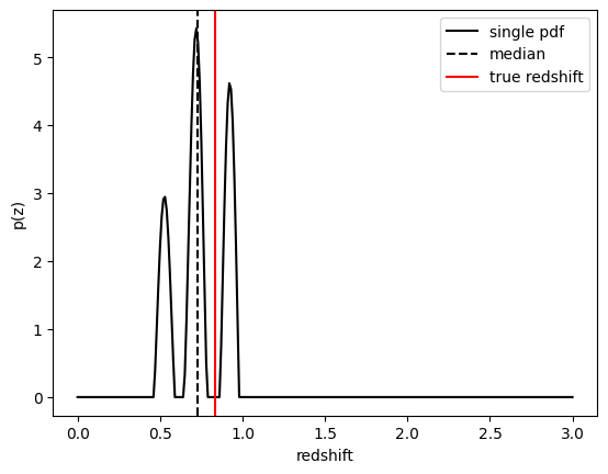
../../../_images/00_Quick_Start_in_Estimation_40_1.png

We can plot an example PDF, its median redshift, and its true redshift from the results file:

galid = 9529
single_gal = np.squeeze(fzresults()[galid].pdf(zgrid))
single_zmedian = fz_medians[galid]
truez = test_data['photometry']['redshift'][galid]
plt.plot(zgrid,single_gal,color='k',label='single pdf')
plt.axvline(single_zmedian,color='k', ls='--', label='median')
plt.axvline(truez,color='r',label='true redshift')
plt.legend(loc='upper right')
plt.xlabel("redshift")
plt.ylabel("p(z)")

Text(0, 0.5, 'p(z)')

../../../_images/00_Quick_Start_in_Estimation_42_1.png

We can also plot a point estimaten against the truth as a visual diagnostic:

plt.figure(figsize=(10,10))
plt.scatter(test_data['photometry']['redshift'],fz_modes,s=1,c='k')
plt.plot([0,3],[0,3],'r--')
plt.xlabel("true redshift")
plt.ylabel("photoz mode")
plt.title("mode point estimate derived from FlexZBoost PDFs");

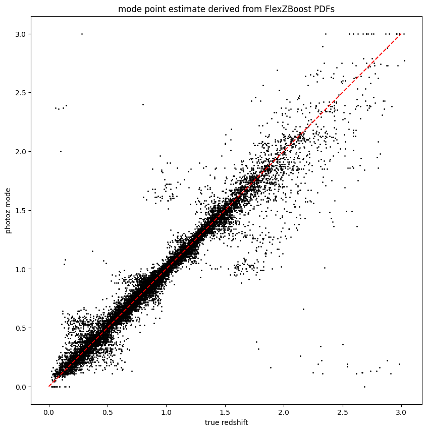
../../../_images/00_Quick_Start_in_Estimation_44_0.png

The results look very good! FlexZBoost is a mature algorithm, and with representative training data we see a very tight correlation with true redshift and few outliers due to physical degeneracies.