Running RAIL with a different dataset

Authors: Sam Schmidt

Last run successfully: September 24, 2025

This is a notebook with a quick example of running a rail algoritm with a different dataset and overriding configuration parameters.

Most of our other demo notebooks use small datasets included with the RAIL demo package, all with the same input names. These datasets are named consistently with many of the default parameter values used in RAIL, e.g. hdf5_groupname="photometry" and ugrizy photometry named in a pattern "mag_{band}_lsst", often specified in SHARED_PARAMS.

This notebook will just show a quick run with an alternate dataset, showing the values that users will likely need to change in order to get things running.

Note: If you’re planning to run this in a notebook, you may want to use interactive mode instead. See Running_with_different_data.ipynb in the interactive_examples/estimation_examples/ folder for a version of this notebook in interactive mode.

import os
import matplotlib.pyplot as plt
import numpy as np
import tables_io

First, we’ll start with grabbing some small datasets from NERSC, a tar file with some data drawn from the Roman-Rubin simulation:

training_file = "./romanrubin_demo_data.tar"

if not os.path.exists(training_file):
  os.system('curl -O https://portal.nersc.gov/cfs/lsst/PZ/romanrubin_demo_data.tar')
  os.system('tar -xvf romanrubin_demo_data.tar')

    % Total    % Received % Xferd  Average Speed   Time    Time     Time  Current
                                   Dload  Upload   Total   Spent    Left  Speed

0     0    0     0    0     0      0      0 --:--:-- --:--:-- --:--:--     0

romanrubin_train_data.hdf5
romanrubin_test_data.hdf5

54 4670k   54 2555k    0     0  2496k      0  0:00:01  0:00:01 --:--:-- 2498k

100 4670k 100 4670k 0 0 4213k 0 0:00:01 0:00:01 –:–:– 4214k

Let’s load one of the files and look at the contents:

infile = "romanrubin_train_data.hdf5"
data = tables_io.read(infile)
data.keys()

odict_keys(['H', 'H_err', 'J', 'J_err', 'g', 'g_err', 'i', 'i_err', 'r', 'r_err', 'redshift', 'u', 'u_err', 'y', 'y_err', 'z', 'z_err'])

We can see that, unlike the demo data in other notebooks, there is no top level hdf5_groupname of “photometry”, the data is directly in the top level of the hdf5 file. As such, we will need to specify hdf5_groupname="" to override the default value of "photometry" in RAIL.

We also see that the magnitudes and errors are simply named with the band name, e.g. "u" rather than "mag_u_lsst". Again, we will need to specify the band and error names in order to override the defaults in RAIL. Let’s do that below, using the KNearNeighInformer and Estimator algorithms:

from rail.core.data import TableHandle
from rail.core.stage import RailStage
from rail.estimation.algos.k_nearneigh import KNearNeighInformer, KNearNeighEstimator

trainFile = "./romanrubin_train_data.hdf5"
testFile = "./romanrubin_test_data.hdf5"
training_data = tables_io.read(trainFile)
test_data = tables_io.read(testFile)
# training_data = DS.read_file("training_data", TableHandle, trainFile)
# test_data = DS.read_file("test_data", TableHandle, testFile)

The dataset-specific parameters

We will need to specify several parameters to override the default values in RAIL, we can create a dictionary of these and pass those into the make_stage for our informer. Because we have Roman J and H, we will also demonstrate running with 8 bands rather than the default six.

RAIL requires that we specify the names of the input columns as bands, and the input errors on those as err_bands. Most algorithms also require a ref_band. To handle non-detections, RAIL uses a dictionary of mag_limits which must contain keys for all of the columns in bands and a float for the value with which the non-detect will be replaced. You may also need to specify a different nondetect_val if the dataset has a different convention for non-detections (in this dataset, our non-detetions have a value of np.inf).

NOTE: RAIL uses SHARED_PARAMS, a central location for specifying a subset of parameters that are common to a dataset, and setting them in one place when running multiple algorithms. However, any configuration parameters specified as SHARED_PARAMS can be overridden in the same way as any other parameter, there is nothing special about them, and we will do that here with bands, err_bands, etc…

Let’s set up our dictionary with these values:

bands = ['u', 'g', 'r', 'i', 'z', 'y', 'J', 'H']
errbands = []
maglims = {}
limvals = [27.8, 29.0, 29.1, 28.6, 28.0, 27.0, 26.4, 26.4]
for band, limval in zip(bands, limvals):
    errbands.append(f"{band}_err")
    maglims[band] = limval


print(bands)
print(errbands)
print(maglims)

['u', 'g', 'r', 'i', 'z', 'y', 'J', 'H']
['u_err', 'g_err', 'r_err', 'i_err', 'z_err', 'y_err', 'J_err', 'H_err']
{'u': 27.8, 'g': 29.0, 'r': 29.1, 'i': 28.6, 'z': 28.0, 'y': 27.0, 'J': 26.4, 'H': 26.4}

knn_dict = dict(hdf5_groupname='', bands=bands, err_bands=errbands, mag_limits=maglims, ref_band='i')

We can now feed this into our inform stage:

pz_train = KNearNeighInformer.make_stage(name='inform_KNN', model='rd_demo_knn.pkl', **knn_dict)

%%time
pz_train.inform(training_data)

Inserting handle into data store.  input: None, inform_KNN

split into 11250 training and 3750 validation samples
finding best fit sigma and NNeigh...

best fit values are sigma=0.017222222222222222 and numneigh=7



Inserting handle into data store.  model_inform_KNN: inprogress_rd_demo_knn.pkl, inform_KNN
CPU times: user 14.1 s, sys: 2.12 s, total: 16.2 s
Wall time: 16.2 s

<rail.core.data.ModelHandle at 0x7f627ee43f70>

We can use the same dictionary to specify overrides for the estimator stage:

pz = KNearNeighEstimator.make_stage(name='KNN', model=pz_train.get_handle('model'), **knn_dict)
results = pz.estimate(test_data)

Inserting handle into data store.  input: None, KNN
Inserting handle into data store.  model_inform_KNN: <class 'rail.core.data.ModelHandle'> rd_demo_knn.pkl, (wd), KNN
Process 0 running estimator on chunk 0 - 20,000
Process 0 estimating PZ PDF for rows 0 - 20,000

Inserting handle into data store.  output_KNN: inprogress_output_KNN.hdf5, KNN

Let’s plot the mode vs the true redshift to make sure that things ran properly:

zmode = results().ancil['zmode'].flatten()

Let’s plot the redshift mode against the true redshifts to see how they look:

plt.figure(figsize=(8,8))
plt.scatter(test_data['redshift'],zmode,s=1,c='k',label='KNN mode')
plt.plot([0,3],[0,3],'r--');
plt.xlabel("true redshift")
plt.ylabel("KNN mode")

Text(0, 0.5, 'KNN mode')

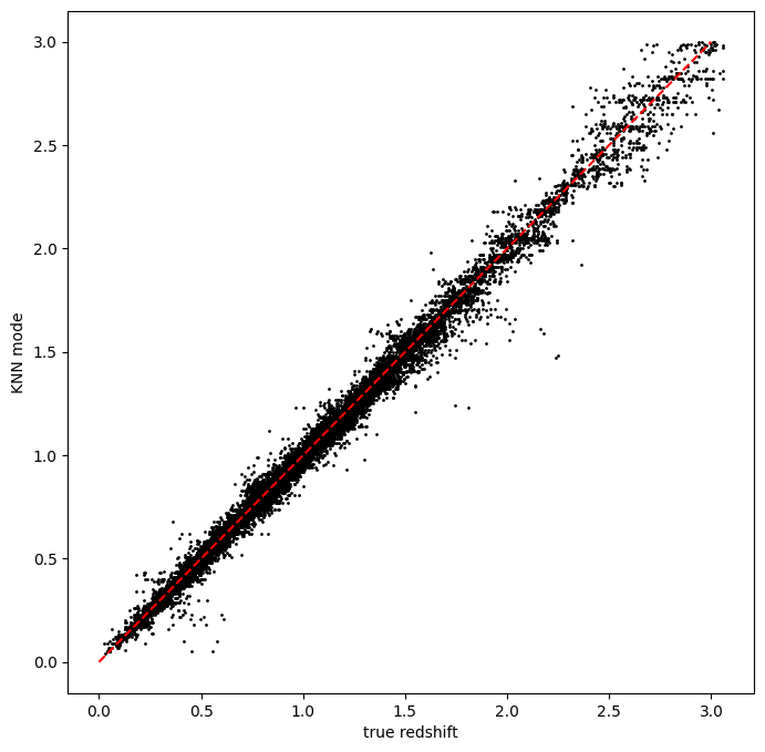
Yes, things look very nice, and the inclusion of NIR photometry gives us very little scatter and very few outliers!