RAIL’s DNF implementation example
Authors: Laura Toribio San Cipriano, Sam Schmidt and Juan De Vicente last successfully run: Feb 05, 2025
This is a notebook demonstrating some of the features of the LSSTDESC
RAIL version of the DNF estimator, see De Vicente et
al. (2016) for more details on the
algorithm.
Note: If you’re planning to run this in a notebook, you may want to
use interactive mode instead. See
DNF.ipynb
in the interactive_examples/estimation_examples/ folder for a
version of this notebook in interactive mode.
DNF (Directional Neighbourhood Fitting) is a nearest-neighbor approach for photometric redshift estimation developed at the CIEMAT (Centro de Investigaciones Energéticas, Medioambientales y Tecnológicas) at Madrid. DNF computes the photo-z hyperplane that best fits the directional neighbourhood of a photometric galaxy in the training sample.
The current version of the code for RAILconsists of a training
stage, DNFInformer and a estimation stage DNFEstimator.
DNFInformer is a class that preprocesses the protometric data,
handles missing or non-detected values, and trains a first basic
k-Nearest Neighbors regressor for redshift prediction. The
DNFEstimator calculates photometric redshifts based on an
enhancement of Nearest Neighbor techniques. The class supports three
main metrics for redshift estimation: ENF, ANF or DNF.
ENF: Euclidean neighbourhood. It’s a common distance metric used in kNN (k-Nearest Neighbors) for photometric redshift prediction.
ANF: uses normalized inner product for more accurate photo-z predictions. It is particularly recommended when working with datasets containing more than four filters.
DNF: combines Euclidean and angular metrics, improving accuracy, especially for larger neighborhoods, and maintaining proportionality in observable content.
DNFInformer
The DNFInformer class processes a training dataset and produces a
model file containing the computed magnitudes, colors, and their
associated errors for the dataset. This model is then utilized in the
DNFEstimator stage for photometric redshift estimation. Missing
photometric detections (non-detections) are handled by replacing them
with a configurable placeholder value, or optionally ignoring them
during model training.
The configurable parameters for DNFInformer include:
bands: List of band names expected in the input dataset.err_bands: List of magnitude error column names corresponding to the bands.redshift_col: String indicating the name of the redshift column in the input data.mag_limits: Dictionary with band names as keys and floats representing the acceptable magnitude range for each band.nondetect_val: Float or np.nan, the value indicating a non-detection, which will be replaced by the values in mag_limits.replace_nondetect: Boolean; if True, non-detections are replaced with the specified nondetect_val. If False, non-detections are ignored during the neighbor-finding process.
DNFEstimator
The DNFEstimator class uses the model generated by DNFInformer to
compute photometric redshifts for new datasets and the PDFs. It
identifies the nearest neighbors from the training data using various
distance metrics and estimates redshifts based on these neighbors.
The configurable parameters for DNFEstimator include:
bands,err_bands,redshift_col,nondetect_val,mag_limits: As described forDNFInformer.selection_mode: Integer indicating the method for neighbor selection:0: Euclidean Neighbourhood Fitting (ENF).1: Angular Neighbourhood Fitting (ANF).2: Directional Neighbourhood Fitting (DNF).
zmin,zmax,nzbins: Float values defining the minimum and maximum redshift range and the number of bins for estimation of the PDFs.pdf_estimation: Boolean; if True, computes a probability density function (PDF) for the redshift of each object.
import os
import matplotlib.pyplot as plt
import numpy as np
#%matplotlib inline
import rail
import qp
import tables_io
from rail.core.data import TableHandle
from rail.core.stage import RailStage
Training the informer
You can configure DNF by setting options in a dictionary when
initializing an instance of our DNFInformer stage. Any parameters
not explicitly defined will use their default values.
dnf_dict = dict(zmin=0.0, zmax=3.0, nzbins=301, hdf5_groupname='photometry')
We will begin by training the algorithm, to to this we instantiate a rail object with a call to the base class.
from rail.estimation.algos.dnf import DNFInformer, DNFEstimator
pz_train = DNFInformer.make_stage(name='inform_DNF', model='demo_DNF_model.pkl', **dnf_dict)
Now, let’s load our training data, which is stored in hdf5 format. We’ll load it into the Data Store so that the ceci stages are able to access it.
from rail.utils.path_utils import RAILDIR
trainFile = os.path.join(RAILDIR, 'rail/examples_data/testdata/test_dc2_training_9816.hdf5')
testFile = os.path.join(RAILDIR, 'rail/examples_data/testdata/test_dc2_validation_9816.hdf5')
training_data = tables_io.read(trainFile)
test_data = tables_io.read(testFile)
The inform stage of DNF transforms magnitudes into colors, corrects undetected values in the training data, and saves them as a model dictionary. This dictionary is then stored in a pickle file specified by the model keyword above, in this case, ‘demo_dnf_model.pkl’.
%%time
pz_train.inform(training_data)
Inserting handle into data store.  input: None, inform_DNF
Inserting handle into data store.  model_inform_DNF: inprogress_demo_DNF_model.pkl, inform_DNF
CPU times: user 9.93 ms, sys: 0 ns, total: 9.93 ms
Wall time: 9.76 ms
<rail.core.data.ModelHandle at 0x7fbae6243be0>
Run DNF
Now, we can configure the main photo-z stage and run our algorithm on
the data to generate basic photo-z estimates. Keep in mind that we are
loading the trained model obtained from the inform stage using the
statementmodel=pz_train.get_handle('model'). We will set
nondetect_replace to True to replace non-detection magnitudes
with their 1-sigma limits and utilize all colors.
DNF provides three methods for selecting the distance metric: Euclidean
(“ENF,” set with selection_mode of 0), Angular (“ANF,” set with
selection_mode = 1, which is the default for this stage), and
Directional (“DNF,” set with selection_mode = 2).
For our first example, we will set selection_mode to 1, using
the angular distance:
%%time
pz = DNFEstimator.make_stage(name='DNF_estimate', hdf5_groupname='photometry',
                        model=pz_train.get_handle('model'),
                        selection_mode=1,
                        nondetect_replace=True)
results = pz.estimate(test_data)
using metric ANF
Inserting handle into data store.  input: None, DNF_estimate
Inserting handle into data store.  model_inform_DNF: <class 'rail.core.data.ModelHandle'> demo_DNF_model.pkl, (wd), DNF_estimate
Process 0 running estimator on chunk 0 - 20,449
Process 0 estimating PZ PDF for rows 0 - 20,449
/opt/hostedtoolcache/Python/3.10.20/x64/lib/python3.10/site-packages/rail/estimation/algos/dnf.py:488: RuntimeWarning: invalid value encountered in sqrt
  alpha = np.sqrt(1.0 - NIP**2)
/opt/hostedtoolcache/Python/3.10.20/x64/lib/python3.10/site-packages/rail/estimation/algos/dnf.py:529: RuntimeWarning: divide by zero encountered in divide
  inverse_distances = 1.0 / distances
/opt/hostedtoolcache/Python/3.10.20/x64/lib/python3.10/site-packages/rail/estimation/algos/dnf.py:537: RuntimeWarning: invalid value encountered in divide
  wmatrix = inverse_distances / row_sum
Inserting handle into data store. output_DNF_estimate: inprogress_output_DNF_estimate.hdf5, DNF_estimate
CPU times: user 3min 1s, sys: 928 ms, total: 3min 2s
Wall time: 3min 2s
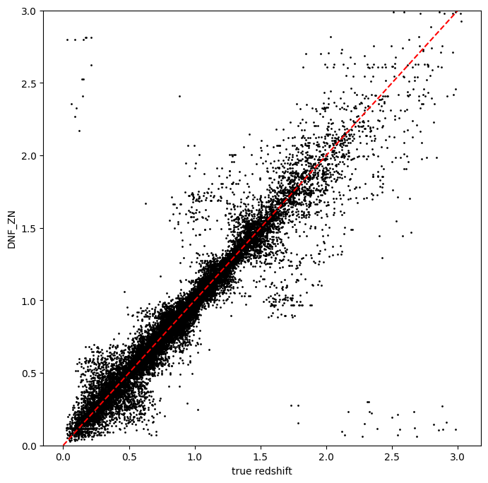
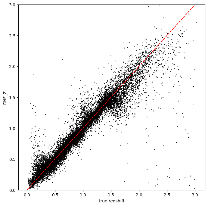
DNF calculates its own point estimate, DNF_Z, which is stored in the
qp Ensemble ancil data. Also, DNF calculates other photo-zs called
DNF_ZN.
DNF_Zrepresents the photometric redshift for each galaxy computed as the weighted average or hyperplane fit (depending on the option selected) for a set of neighbors determined by a specific metric (ENF, ANF, DNF) where the outliers are removedDNF_ZNrepresents the photometric redshift using only the closest neighbor. It is mainly used for computing the redshift distributions.
Let’s plot that versus the true redshift. We can also compute the PDF mode for each object and plot that as well:
zdnf = results().ancil['DNF_Z'].flatten()
zn_dnf = results().ancil['DNF_ZN'].flatten()
zgrid = np.linspace(0,3,301)
zmode = results().mode(zgrid).flatten()
zmode
array([0.08, 0.03, 0.03, ..., 3. , 2.94, 3. ], shape=(20449,))
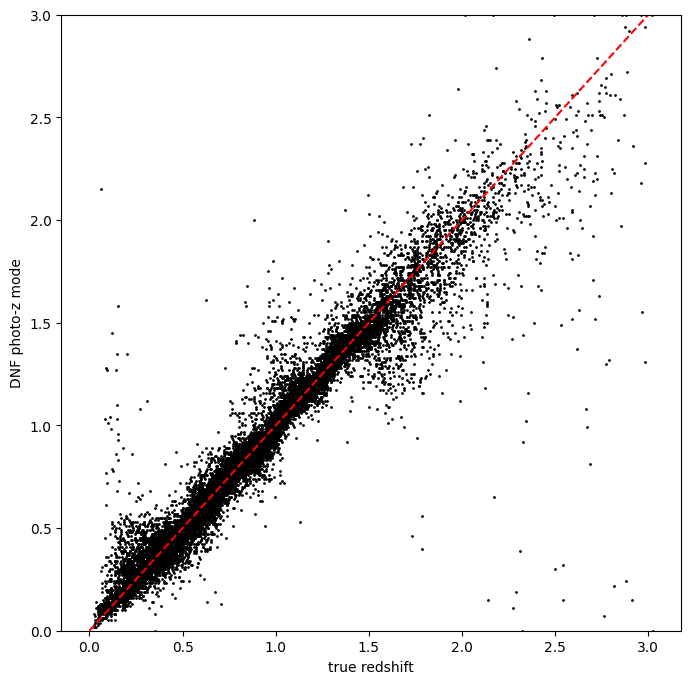
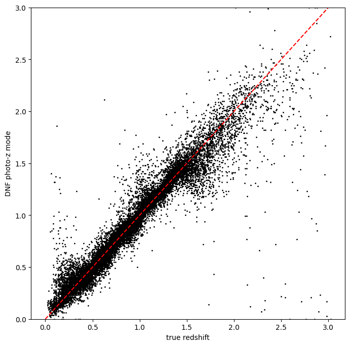
Let’s plot the redshift mode against the true redshifts to see how they look:
plt.figure(figsize=(8,8))
plt.scatter(test_data['photometry']['redshift'],zmode,s=1,c='k',label='DNF mode')
plt.plot([0,3],[0,3],'r--');
plt.xlabel("true redshift")
plt.ylabel("DNF photo-z mode")
plt.ylim(0,3)
(0.0, 3.0)
plt.figure(figsize=(8,8))
plt.scatter(test_data['photometry']['redshift'], zdnf, s=1, c='k')
plt.plot([0,3],[0,3], 'r--');
plt.xlabel("true redshift")
plt.ylabel("DNF_Z")
plt.ylim(0,3)
(0.0, 3.0)

plt.figure(figsize=(8,8))
plt.scatter(test_data['photometry']['redshift'], zn_dnf, s=1, c='k')
plt.plot([0,3],[0,3], 'r--');
plt.xlabel("true redshift")
plt.ylabel("DNF_ZN")
plt.ylim(0,3)
(0.0, 3.0)
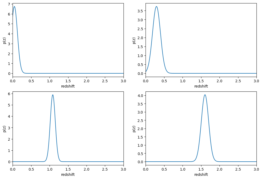
plotting PDFs
In addition to point estimates, we can also plot a few of the full PDFs
produced by DNF using the plot_native method of the qp Ensemble that
we’ve created as results. We can specify which PDF to plot with the
key argument to plot_native, let’s plot four, the 5th, 1380th,
14481st, and 18871st:
fig, axs = plt.subplots(2, 2, figsize=(12,8))
whichgals = [4, 1379, 14480, 18870]
for ax, which in zip(axs.flat, whichgals):
    ax.set_xlim(0,3)
    results().plot_native(key=which, axes=ax)
    ax.set_xlabel("redshift")
    ax.set_ylabel("p(z)")
Other distance metrics
Besides DNF there are options for ENF and ANF.
Let’s run our estimator using selection_mode=0 for the Euclidean
distance, and compare both the mode results and PDF results:
%%time
pz2 = DNFEstimator.make_stage(name='DNF_estimate2', hdf5_groupname='photometry',
                        model=pz_train.get_handle('model'),
                        selection_mode=0,
                        nondetect_replace=True)
results2 = pz2.estimate(test_data)
using metric ENF
Inserting handle into data store.  input: None, DNF_estimate2
Inserting handle into data store.  model_inform_DNF: <class 'rail.core.data.ModelHandle'> demo_DNF_model.pkl, (wd), DNF_estimate2
Process 0 running estimator on chunk 0 - 20,449
Process 0 estimating PZ PDF for rows 0 - 20,449
Inserting handle into data store. output_DNF_estimate2: inprogress_output_DNF_estimate2.hdf5, DNF_estimate2
CPU times: user 3min 9s, sys: 1.18 s, total: 3min 10s
Wall time: 3min 10s
zdnf2 = results2().ancil['DNF_Z'].flatten()
zgrid = np.linspace(0,3,301)
zmode2 = results2().mode(zgrid).flatten()
plt.figure(figsize=(8,8))
plt.scatter(test_data['photometry']['redshift'],zmode2,s=1,c='k',label='DNF mode')
plt.plot([0,3],[0,3],'r--');
plt.xlabel("true redshift")
plt.ylabel("DNF photo-z mode")
plt.ylim(0,3)
(0.0, 3.0)
plt.figure(figsize=(8,8))
plt.scatter(test_data['photometry']['redshift'], zdnf2, s=1, c='k')
plt.plot([0,3],[0,3], 'r--');
plt.xlabel("true redshift")
plt.ylabel("DNF_Z")
plt.ylim(0,3)
(0.0, 3.0)
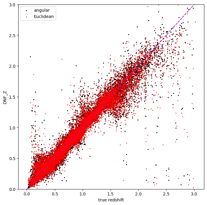
Let’s directly compare the “angular” and “Euclidean” distance estimates on the same axes:
plt.figure(figsize=(8,8))
plt.scatter(test_data['photometry']['redshift'], zdnf, s=2, c='k', label="angular")
plt.scatter(test_data['photometry']['redshift'], zdnf2, s=1, c='r', label="Euclidean")
plt.legend(loc='upper left', fontsize=10)
plt.plot([0,3],[0,3], 'm--');
plt.xlabel("true redshift")
plt.ylabel("DNF_Z")
plt.ylim(0,3)
(0.0, 3.0)
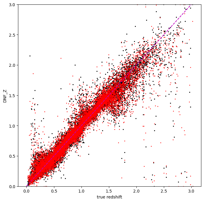
plt.figure(figsize=(8,8))
plt.scatter(test_data['photometry']['redshift'], zmode, s=2, c='k')
plt.scatter(test_data['photometry']['redshift'], zmode2, s=1, c='r')
plt.plot([0,3],[0,3], 'm--');
plt.xlabel("true redshift")
plt.ylabel("DNF_Z")
plt.ylim(0,3)
(0.0, 3.0)
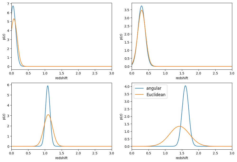
Finally, let’s directly compare the same PDFs that we plotted above
fig, axs = plt.subplots(2, 2, figsize=(12,8))
whichgals = [4, 1379, 14480, 18870]
for ax, which in zip(axs.flat, whichgals):
    ax.set_xlim(0,3)
    results().plot_native(key=which, axes=ax, label="angular")
    results2().plot_native(key=which, axes=ax, label="Euclidean")
    ax.set_xlabel("redshift")
    ax.set_ylabel("p(z)")
ax.legend(loc='upper left', fontsize=12)
<matplotlib.legend.Legend at 0x7fbacd936ce0>