RAIL CMNN Tutorial Notebook
Author: Sam Schmidt
Last Successfully Run: September 26, 2023
Note: If you’re planning to run this in a notebook, you may want to
use interactive mode instead. See
CMNN.ipynb
in the interactive_examples/estimation_examples/ folder for a
version of this notebook in interactive mode.
This is a notebook demonstrating some of the features of the LSSTDESC
RAIL version of the CMNN estimator, see Graham et
al. (2018)
for more details on the algorithm.
CMNN stands for color-matched nearest-neighbor, and as this name implies, the method works by finding the Mahalanobis distance between each test galaxy and the training galaxies, and selecting one of those “nearby” in color space as the redshift estimate. The algorithm also estimates the “width” of the resulting PDF based on the standard deviation of this nearby set and returns a single Gaussian with a mean and width defined as such.
The current version of the code consists of a training stage,
CMNNInformer, that computes colors for a set of training data and an
estimation stage CMNNEstimator that calculates the Mahalanobis
distance to each training galaxy for each test galaxy and returns a
single Guassian PDF for each galaxy. The mean value of this Gaussian PDF
can be estimated in one of three ways (see selection mode below), and
the width is determined by the standard deviation of training galaxy
redshifts within the threshold Mahalanobis distance. Future
implementation improvements may change the output format to include
multiple Gaussians.
For the color calculation, there is an option for how to treat the
“non-detections” in a band: the default choice is to ignore any colors
that contain a non-detect magnitude and adjust the number of degrees of
freedom in the Mahalanobis distance accordingly (this is how the CMNN
algorithm was originally implemented). Or, if the configuration
parameter nondetect_replace is set to True in CMNNInformer,
the non-detected magnitudes will be replaced with the 1-sigma limiting
magnitude in each band as supplied by the user via the mag_limits
configuration parameter (or by the default 1-sigma limits if the user
does not supply specific numbers). We have not done any exploration of
the relative performance of these two choices, but note that there is
not a significant performance difference in terms of runtime between the
two methods.
In addition to the Gaussian PDF for each test galaxy, two ancillary
quantities are stored: zmode: the mode of the redshift PDF and
Ncm, the integer number of “nearby” galaxies considered as neighbors
for each galaxy.
CMNNInformer takes in a training data set and returns a model file
that simply consists of the computed colors and color errors (magnitude
errors added in quadrature) for that dataset, the model to be used in
the CMNNEstimator stage. A modification of the original CMNN
algorithm, “nondetections” are now replaced by the 1-sigma limiting
magnitudes and the non-detect magnitude errors replaced with a value of
1.0. The config parameters that can be set by the user for
CMNNInformer are:
bands: list of the band names that should be present in the input data.
err_bands: list of the magnitude error column names that should be present in the input data.
redshift_col: a string giving the name for the redshift column present in the input data.
mag_limits: a dictionary with keys that match those in bands and a float with the 1 sigma limiting magnitude for each band.
nondetect_val: float or np.nan, the value indicating a non-detection, which will be replaced by the values in mag_limits.
nondetect_replace: bool, if set to
False(the default) this option ignores colors with non-detected values in the Mahalanobis distance calculation, with a corresponding drop in the degrees of freedom value. If set toTrue, the method will replace non-detections with the 1-sigma limiting magnitudes specified viamag_limits(or default 1-sigma limits if not supplied), and will use all colors in the Mahalanobis distance calculation.
The parameters that can be set via the config_params in
CMNNEstimator are described in brief below:
bands, err_bands, redshift_col, mag_limits are all the same as described above for CMNNInformer.
ppf_value: float, usually 0.68 or 0.95, which sets the value of the PPF used in the Mahalanobis distance calculation.
selection_mode: int, selects how the central value of the Gaussian PDF is calculated in the algorithm, if set to 0 randomly chooses from set within the Mahalanobis distance, if set to 1 chooses the nearest neighbor point, if set to 2 adds a distance weight to the random choice.
min_n: int, the minimum number of training galaxies to use.
min_thresh: float, the minimum threshold cutoff. Values smaller than this threshold value will be ignored.
min_dist: float, the minimum Mahalanobis distance. Values smaller than this will be ignored.
bad_redshift_val: float, in the unlikely case that there are not enough training galaxies, this central redshift will be assigned to galaxies.
bad_redshift_err: float, in the unlikely case that there are not enough training galaxies, this Gaussian width will be assigned to galaxies.
Let’s grab some example data, train the model by running the
CMNNInformer inform method, then calculate a set of photo-z’s
using CMNNEstimator estimate. Much of the following is copied
from the 00_Quick_Start_in_Estimation.ipynb in the RAIL repo, so
look at that notebook for general questions on setting up the RAIL
infrastructure for estimators.
import os
import matplotlib.pyplot as plt
import numpy as np
%matplotlib inline
import rail
import qp
import tables_io
from rail.core.data import TableHandle
from rail.core.stage import RailStage
Getting the list of available Estimators
RailStage knows about all of the sub-types of stages. The are stored in
the RailStage.pipeline_stages dict. By looping through the values in
that dict we can and asking if each one is a sub-class of
rail.estimation.estimator.CatEstimator we can identify the available
estimators that operator on catalog-like inputs.
The code-specific parameters
As mentioned above, CMNN has particular configuration options that can
be set when setting up an instance of our CMNNInformer stage, we’ll
define those in a dictionary. Any parameters not specifically assigned
will take on default values.
cmnn_dict = dict(zmin=0.0, zmax=3.0, nzbins=301, hdf5_groupname='photometry')
We will begin by training the algorithm, to to this we instantiate a rail object with a call to the base class.
from rail.estimation.algos.cmnn import CMNNInformer, CMNNEstimator
pz_train = CMNNInformer.make_stage(name='inform_CMNN', model='demo_cmnn_model.pkl', **cmnn_dict)
Now, let’s load our training data, which is stored in hdf5 format. We’ll load it into the Data Store so that the ceci stages are able to access it.
from rail.utils.path_utils import RAILDIR
trainFile = os.path.join(RAILDIR, 'rail/examples_data/testdata/test_dc2_training_9816.hdf5')
testFile = os.path.join(RAILDIR, 'rail/examples_data/testdata/test_dc2_validation_9816.hdf5')
training_data = tables_io.read(trainFile)
test_data = tables_io.read(testFile)
The inform stage for CMNN should not take long to run, it essentially
just converts the magnitudes to colors for the training data and stores
those as a model dictionary which is stored in a pickle file specfied by
the model keyword above, in this case “demo_cmnn_model.pkl”. This
file should appear in the directory after we run the inform stage in the
cell below:
%%time
pz_train.inform(training_data)
Inserting handle into data store.  input: None, inform_CMNN
Inserting handle into data store.  model_inform_CMNN: inprogress_demo_cmnn_model.pkl, inform_CMNN
CPU times: user 293 μs, sys: 2.03 ms, total: 2.32 ms
Wall time: 2.06 ms
<rail.core.data.ModelHandle at 0x7fd4b489f3a0>
We can now set up the main photo-z stage and run our algorithm on the
data to produce simple photo-z estimates. Note that we are loading the
trained model that we computed from the inform stage: with the
model=pz_train.get_handle('model') statement. We will set
nondetect_replace to True to replace our non-detection
magnitudes with their 1-sigma limits and use all colors.
Let’s also set the minumum number of neighbors to 24, and the
selection_mode to “1”, which will choose the nearest neighbor for
each galaxy as the redshift estimate:
%%time
pz = CMNNEstimator.make_stage(name='CMNN', hdf5_groupname='photometry',
                        model=pz_train.get_handle('model'),
                        min_n=20,
                        selection_mode=1,
                        nondetect_replace=True,
                        aliases={"output":"pz_near"})
results = pz.estimate(test_data)
Inserting handle into data store.  input: None, CMNN
Inserting handle into data store.  model_inform_CMNN: <class 'rail.core.data.ModelHandle'> demo_cmnn_model.pkl, (wd), CMNN
Process 0 running estimator on chunk 0 - 20,449
Process 0 estimating PZ PDF for rows 0 - 20,449
Inserting handle into data store.  output_CMNN: inprogress_output_CMNN.hdf5, CMNN
CPU times: user 48 s, sys: 7.43 ms, total: 48 s
Wall time: 48 s
As mentioned above, in addition to the PDF, estimate calculates and
stores both the mode of the PDF (zmode), and the number of neighbors
(Ncm) for each galaxy, which can be accessed from the ancillary
data. We will plot the modes vs the true redshift to see how well CMNN
did in estimating redshifts:
zmode = results().ancil['zmode']
Let’s plot the redshift mode against the true redshifts to see how they look:
plt.figure(figsize=(8,8))
plt.scatter(test_data['photometry']['redshift'],zmode,s=1,c='k',label='simple NN mode')
plt.plot([0,3],[0,3],'r--');
plt.xlabel("true redshift")
plt.ylabel("CMNN photo-z mode")
plt.ylim(0,3)
(0.0, 3.0)
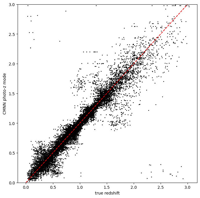
Very nice! Not many outliers and a fairly small scatter without much bias!
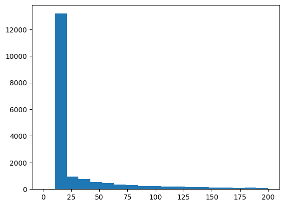
Now, let’s plot the histogram of how many neighbors were used. We set a minimum number of 20, so we should see a large peak at that value:
ncm =results().ancil['Ncm']
plt.hist(ncm, bins=np.linspace(0,200,20));
As mentioned previously, we can change the method for how we select the
mean redshift, let’s re-run the estimator but use selection_mode =
“0”, which will select a random galaxy from amongst the neighbors. This
should still look decent, but perhaps not as nice as the nearest
neighbor estimator:
pz_rand = CMNNEstimator.make_stage(name='CMNN_rand', hdf5_groupname='photometry',
                             model=pz_train.get_handle('model'),
                             min_n=20,
                             selection_mode=0,
                             nondetect_replace=True,
                             aliaes={"output": "pz_rand"})
results_rand = pz_rand.estimate(test_data)
Inserting handle into data store.  input: None, CMNN_rand
Inserting handle into data store.  model_inform_CMNN: <class 'rail.core.data.ModelHandle'> demo_cmnn_model.pkl, (wd), CMNN_rand
Process 0 running estimator on chunk 0 - 20,449
Process 0 estimating PZ PDF for rows 0 - 20,449
Inserting handle into data store. output_CMNN_rand: inprogress_output_CMNN_rand.hdf5, CMNN_rand
zmode_rand = results_rand().ancil['zmode']
plt.figure(figsize=(8,8))
plt.scatter(test_data['photometry']['redshift'],zmode_rand,s=1,c='k',label='simple NN mode')
plt.plot([0,3],[0,3],'r--');
plt.xlabel("true redshift")
plt.ylabel("CMNN photo-z mode")
plt.ylim(0,3)
(0.0, 3.0)
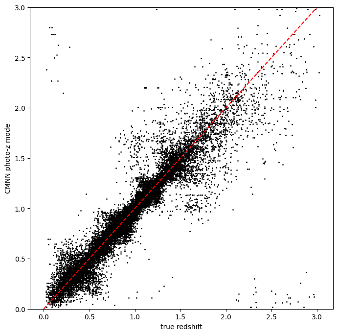
Slightly worse, but not dramatically so, a few more outliers are visible
visually. Finally, we can try the weighted random selection by setting
selection_mode to “2”:
pz_weight = CMNNEstimator.make_stage(name='CMNN_weight', hdf5_groupname='photometry',
                               model=pz_train.get_handle('model'),
                               min_n=20,
                               selection_mode=2,
                               nondetect_replace=True,
                               aliaes={"output": "pz_weight"})
results_weight = pz_weight.estimate(test_data)
Inserting handle into data store.  input: None, CMNN_weight
Inserting handle into data store.  model_inform_CMNN: <class 'rail.core.data.ModelHandle'> demo_cmnn_model.pkl, (wd), CMNN_weight
Process 0 running estimator on chunk 0 - 20,449
Process 0 estimating PZ PDF for rows 0 - 20,449
Inserting handle into data store. output_CMNN_weight: inprogress_output_CMNN_weight.hdf5, CMNN_weight
zmode_weight = results_weight().ancil['zmode']
plt.figure(figsize=(8,8))
plt.scatter(test_data['photometry']['redshift'],zmode_weight,s=1,c='k',label='simple NN mode')
plt.plot([0,3],[0,3],'r--');
plt.xlabel("true redshift")
plt.ylabel("CMNN photo-z mode")
plt.ylim(0,3)
(0.0, 3.0)

Again, not a dramatic difference, but it can make a difference if there is sparse coverage of areas of the color-space by the training data, where choosing “nearest” might choose the same single data point for many test points, whereas setting to random or weighted random could slightly “smooth” that choice by forcing choices of other nearby points for the redshift estimate.
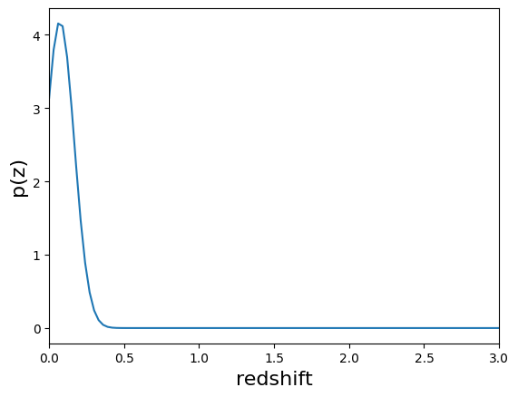
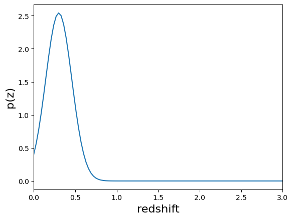
Finally, let’s plot a few PDFs, again, they are a single Gaussian:
results().plot_native(key=9, xlim=(0,3))
<Axes: xlabel='redshift', ylabel='p(z)'>
results().plot_native(key=1554, xlim=(0,3))
<Axes: xlabel='redshift', ylabel='p(z)'>
results().plot_native(key=19554, xlim=(0,3))
<Axes: xlabel='redshift', ylabel='p(z)'>
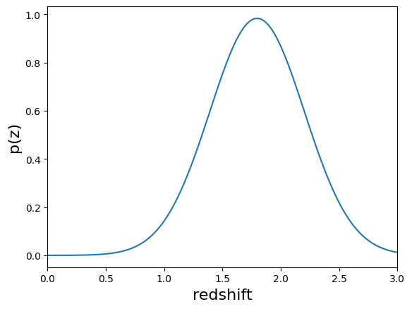
We see a wide variety of widths, as expected for a single Gaussian parameterization that must encompass a wide variety of PDF shapes.