Clustering redshifts with yet_another_wizz

This notebooks summarises the steps to compute clustering redshifts for an unknown sample of galaxies using a reference sample with known redshifts. Additionally, a correction for the galaxy bias of the reference sample is applied (see Eqs. 17 & 20 in van den Busch et al. 2020).

This involves a number of steps (see schema below): 1. Preparing the input data (creating randoms, applying masks; simplfied here). 2. Splitting the data into spatial patches and cache them on disk for faster access. 3. Computing the autocorrelation function amplitude \(w_{\rm ss}(z)\), used as correction for the galaxy bias 4. Computing the cross-correlation function amplitude \(w_{\rm sp}(z)\), which is the biased redshift estimate. 5. Summarising the result by correcting for the refernece sample bias and producing a redshift estimate (not a PDF!).

Note: The cached data must be removed manually since its lifetime can currently not be handled by RAIL.

The aim of this notebook is to give an overview of the wrapper functionality, including a summary of all currently implemented optional parameters (commented). It is not meant to be a demonstaration of the performance of yet_another_wizz since the example data used here is very small and the resulting signal-to-noise ratio is quite poor.

Note: If you’re planning to run this in a notebook, you may want to use interactive mode instead. See YAW.ipynb in the interactive_examples/estimation_examples/ folder for a version of this notebook in interactive mode.

import matplotlib.pyplot as plt

from rail.core.data import TableHandle, Hdf5Handle

from rail.core.stage import RailStage
import tables_io

# step 1
from yaw.randoms import BoxRandoms
from rail.yaw_rail.utils import get_dc2_test_data

from rail.estimation.algos.cc_yaw import (
    create_yaw_cache_alias,  # utility for YawCacheCreate
    YawCacheCreate,     # step 2
    YawAutoCorrelate,   # step 3
    YawCrossCorrelate,  # step 4
    YawSummarize,       # step 5
)  # equivalent: from rail.yaw_rail import *

VERBOSE = "debug"  # verbosity level of built-in logger, disable with "error"

1. Data preparation

Since this is a simple example, we are not going into the details of creating realistic randoms and properly masking the reference and unknown data to a shared footprint on sky. Instead, we are using a simulated dataset that serves as both, reference and unknown sample.

First, we download the small test dataset derived from 25 sqdeg of DC2, containing 100k objects on a limited redshift range of \(0.2 < z < 1.8\). We add the data as new handle to the datastore.

test_data = get_dc2_test_data()  # downloads test data, cached for future calls
redshifts = test_data["z"].to_numpy()
zmin = redshifts.min()
zmax = redshifts.max()
n_data = len(test_data)
print(f"N={n_data}, {zmin:.1f}<z<{zmax:.1f}")

handle_test_data = Hdf5Handle("input_data",data=test_data)

N=100000, 0.2<z<1.8

Next we generate a x10 enhanced uniform random dataset for the test data constrained to its rectangular footprint. We add redshifts by cloning the redshift column "z" of the dataset. We add the randoms as new handle to the datastore.

generator = BoxRandoms(
    test_data["ra"].min(),
    test_data["ra"].max(),
    test_data["dec"].min(),
    test_data["dec"].max(),
    redshifts=redshifts,
    seed=12345,
)
test_rand = generator.generate_dataframe(n_data * 10)
test_rand.rename(columns=dict(redshifts="z"), inplace=True)

handle_test_rand = Hdf5Handle("input_rand", data=test_rand)

2. Splitting and caching the data

This step is crucial to compute consistent clustering redshift uncertainties. yet_another_wizz uses spatial (jackknife) resampling and therefore, every input dataset must be split into the same exact spatial regions/patches. To improve the parallel performance, the datasets and randoms are pre-arranged into these patches and cached on disk for better random patch-wise access. While this is slow for small datasets, it is highly beneficial for large datasets with many patches and/or memory constraints.

The RAIL wrapper uses manually specified cache directories, each of which contains one dataset and optionally corresponding randoms. This ensures that the patch centers are defined consistently. To create a new cache, use the YawCacheCreate.create() method.

Note on names and aliasing in RAIL

We need to create separate caches for the reference and the unknown data, which means that we need to run the YawCacheCreate twice. Since that creates name clashes in the RAIL datastore, we need to properly alias the inputs (data/ rand) and the output (cache) by providing a dictionary for the aliases parameter when calling the make_stage(), e.g. by adding a unique suffix:

name = "stage_name"
aliases = dict(data="data_suffix", rand="rand_suffix", cache="cache_suffix")

There is a shorthand for convenience (from rail.yaw_rail.cache.AliasHelper) that allows to generate this dictionary by just providing a suffix name for the stage instance (see example below).

name = "stage_name"
aliases = create_yaw_cache_alias("suffix")

The reference data

To create a cache directory we must specify a path to the directory at which the data will be cached. This directory must not exist yet. We also have to specify a name for the stage to ensure that the reference and unknown caches (see below) are properly aliased to be distinguishable by the RAIL datastore.

Furthermore, a few basic column names that describe the tabular input data must be provided. These are right ascension (ra_name) and declination (dec_name), and in case of the reference sample also the redshifts (redshift_name). Finally, the patches must be defined and there are three ways to do so: 1. Stage parameter patch_file: Read the patch center coordinates from an ASCII file with pairs of R.A/Dec. coordinates in radian. 2. Stage parameter patch_num: Generating a given number of patches from the object positions (peferrably of the randoms if possible) using k-means clustering. 3. Stage parameter patch_name: Providing a column name in the input table which contains patch indices (using 0-based indexing). 4. Stage input patch_source: Using the patch centers from a different cache instance, given by a cache handle. When this input is provided it takes precedence over any of the stage parameters above.

In this example we choose to auto-generate five patches. In a more realistic setup this number should be much larger.

stage_cache_ref = YawCacheCreate.make_stage(
    name="cache_ref",
    aliases=create_yaw_cache_alias("ref"),
    path="run/test_ref",
    overwrite=True,  # default: False
    ra_name="ra",
    dec_name="dec",
    redshift_name="z",
    # weight_name=None,
    # patch_name=None,
    patch_num=5,  # default: None
    # max_workers=None,
    verbose=VERBOSE,  # default: "info"
)
handle_cache_ref = stage_cache_ref.create(
    data=handle_test_data,
    rand=handle_test_rand,
    # patch_source=None,
)

Inserting handle into data store.  data_ref: None, cache_ref
Inserting handle into data store.  rand_ref: None, cache_ref
YAW | yet_another_wizz v3.1.2

INF | running in multiprocessing environment with 2 workers

Inserting handle into data store.  patch_source_ref: None, cache_ref
INF | loading 1M records in 1 chunks from memory

DBG | selecting input columns: ra, dec, z

DBG | creating 5 patches

INF | computing 5 patch centers from subset of 224K records

DBG | running preprocessing on 2 workers

INF | using cache directory: run/test_ref/rand

INF | computing patch metadata

DBG | running parallel jobs on 2 workers

INF | loading 100K records in 1 chunks from memory

DBG | selecting input columns: ra, dec, z

DBG | applying 5 patches

DBG | running preprocessing on 2 workers

INF | using cache directory: run/test_ref/data

INF | computing patch metadata

DBG | running parallel jobs on 2 workers

Inserting handle into data store.  output_cache_ref: inprogress_output_cache_ref.path, cache_ref

We can see from the log messages that yet_another_wizz processes the randoms first and generates patch centers (creating 5 patches) and then applies them to the dataset, which is processed last (applying 5 patches). Caching the data can take considerable time depending on the hardware and the number of patches.

The unknown data

The same procedure for the unknown sample, however there are some small, but important differences. We use a different path and name, do not specify the redshift_name (since we would not have this information with real data), and here we chose to not provide any randoms for the unknown sample and instead rely on the reference sample randoms for cross-correlation measurements.

Most importantly, we must ensure that the patch centers are consistent with the reference data and therefore provide the reference sample cache as a stage input called patch_source.

Important: Even if the reference and unknown data are the same as in this specific case, the automatically generated patch centers are not deterministic. We can see in the log messages that the code reports applying 5 patches.

stage_cache_unk = YawCacheCreate.make_stage(
    name="cache_unk",
    aliases=create_yaw_cache_alias("unk"),
    path="run/test_unk",
    overwrite=True,  # default: False
    ra_name="ra",
    dec_name="dec",
    # redshift_name=None,
    # weight_name=None,
    # patch_name=None,
    # patch_num=None,
    # max_workers=None,
    verbose=VERBOSE,  # default: "info"
)
handle_cache_unk = stage_cache_unk.create(
    data=handle_test_data,
    # rand=None,
    patch_source=handle_cache_ref,
)

Inserting handle into data store.  data_unk: None, cache_unk
Inserting handle into data store.  patch_source_unk: None, cache_unk
YAW | yet_another_wizz v3.1.2

INF | running in multiprocessing environment with 2 workers

Inserting handle into data store.  rand_unk: None, cache_unk
INF | loading 100K records in 1 chunks from memory

DBG | selecting input columns: ra, dec

DBG | applying 5 patches

DBG | running preprocessing on 2 workers

INF | using cache directory: run/test_unk/data

INF | computing patch metadata

DBG | running parallel jobs on 2 workers

Inserting handle into data store.  output_cache_unk: inprogress_output_cache_unk.path, cache_unk

3. Computing the autocorrelation / bias correction

The bias correction is computed from the amplitude of the angular autocorrelation function of the reference sample. The measurement parameters are the same as for the cross-correlation amplitude measurement, so we can define all configuration parameters once in a dictionary.

As a first step, we need to decide on which redshift bins/sampling we want to compute the clustering redshifts. Here we choose the redshift limits of the reference data (zmin/zmax) and, since the sample is small, only 8 bins (zbin_num) spaced linearly in redshift (default method="linear"). Finally, we have to define the physical scales in kpc (rmin/rmax, converted to angular separation at each redshift) on which we measure the correlation amplitudes.

Optional parameters: Bins edges can alternatively specifed manually through zbins. To apply scale dependent weights, e.g. \(w \propto r^{-1}\), specify the power-law exponent asrweight=-1. The parameter resolution specifies the radial resolution (logarithmic) of the weights.

corr_config = dict(
    rmin=100,   # in kpc
    rmax=1000,  # in kpc
    # rweight=None,
    # resolution=50,
    zmin=zmin,
    zmax=zmax,
    num_bins=8,  # default: 30
    # method="linear",
    # edges=np.linspace(zmin, zmax, zbin_num+1)
    # closed="right",
    # max_workers=None,
    verbose=VERBOSE,  # default: "info"
)

We then measure the autocorrelation using the YawAutoCorrelate.correlate() method, which takes a single parameter, the cache (handle) of the reference dataset.

stage_auto_corr = YawAutoCorrelate.make_stage(
    name="auto_corr",
    **corr_config,
)
handle_auto_corr = stage_auto_corr.correlate(
    sample=handle_cache_ref,
)

Inserting handle into data store.  output_cache_ref: None, auto_corr
YAW | yet_another_wizz v3.1.2

INF | running in multiprocessing environment with 2 workers

INF | building data trees

DBG | building patch-wise trees (using 8 bins)

DBG | running parallel jobs on 2 workers

INF | building random trees

DBG | building patch-wise trees (using 8 bins)

DBG | running parallel jobs on 2 workers

INF | computing auto-correlation from DD, DR, RR

DBG | computing patch linkage with max. separation of 1.42e-03 rad

DBG | created patch linkage with 19 patch pairs

DBG | using 1 scales without weighting

INF | counting DD from patch pairs

DBG | running parallel jobs on 2 workers

INF | counting DR from patch pairs

DBG | running parallel jobs on 2 workers

INF | counting RR from patch pairs

DBG | running parallel jobs on 2 workers

Inserting handle into data store.  output_auto_corr: inprogress_output_auto_corr.hdf5, auto_corr

As the code is progressing, we can observe the log messages of yet_another_wizz which indicate the performed steps: getting the cached data, generating the job list of patches to correlate, and counting pairs. Finally, the pair counts are stored as custom data handle in the datastore.

We can interact with the returned pair counts (yaw.CorrFunc, documentation) manually if we want to investigate the results:

counts_auto = handle_auto_corr.data  # extract payload from handle
counts_auto.dd

NormalisedCounts(auto=True, binning=8 bins @ (0.200...1.800], num_patches=5)

4. Computing the cross-correlation / redshift estimate

The cross-correlation amplitude, which is the biased estimate of the unknown redshift distribution, is computed similarly to the autocorrelation above. We measure the correlation using the YawCrossCorrelate.correlate() method, which takes two parameters, the cache (handles) of the reference and the unknown data.

stage_cross_corr = YawCrossCorrelate.make_stage(
    name="cross_corr",
    **corr_config,
)
handle_cross_corr = stage_cross_corr.correlate(
    reference=handle_cache_ref,
    unknown=handle_cache_unk,
)

Inserting handle into data store.  output_cache_ref: None, cross_corr
Inserting handle into data store.  output_cache_unk: None, cross_corr
YAW | yet_another_wizz v3.1.2

INF | running in multiprocessing environment with 2 workers

INF | building reference data trees

DBG | building patch-wise trees (using 8 bins)

DBG | running parallel jobs on 2 workers

INF | building reference random trees

DBG | building patch-wise trees (using 8 bins)

DBG | running parallel jobs on 2 workers

INF | building unknown data trees

DBG | building patch-wise trees (unbinned)

DBG | running parallel jobs on 2 workers

INF | computing cross-correlation from DD, RD

DBG | computing patch linkage with max. separation of 1.42e-03 rad

DBG | created patch linkage with 19 patch pairs

DBG | using 1 scales without weighting

INF | counting DD from patch pairs

DBG | running parallel jobs on 2 workers

INF | counting RD from patch pairs

DBG | running parallel jobs on 2 workers

Inserting handle into data store.  output_cross_corr: inprogress_output_cross_corr.hdf5, cross_corr

As before, we can see the actions performed by yet_another_wizz. The main difference for the cross-correlation function is that the second sample (the unknown data/randoms) are not binned by redshift when counting pairs.

As for the autocorrelation, we can interact with the result, e.g. by evaluating the correlation estimator manually and getting the cross-correlation amplitude per redshift bin.

counts_cross = handle_cross_corr.data  # extract payload from handle
corrfunc = counts_cross.sample()  # evaluate the correlation estimator
corrfunc.data

DBG | sampling correlation function with estimator 'DP'

array([0.0023559 , 0.00403239, 0.00684468, 0.01126758, 0.00945143,
       0.00898257, 0.00882812, 0.01273689])

5. Computing the redshift estimate

The final analysis step is combining the two measured correlation amplitudes to get a redshift estimate which is corrected for the reference sample bias. This estimate is not a PDF. Converting the result to a proper PDF (without negative values) is non-trivial and requires further modelling stages that are currently not part of this wrapper.

We use YawSummarize.summarize() method, which takes the pair count handles of the cross- and autocorrelation functions as input. In principle, the autocorrelation of the unknown sample could be specified to fully correct for galaxy bias, however this is not possible in practice since the exact redshifts of the unknown objects are not known.

stage_summarize = YawSummarize.make_stage(
    name="summarize",
    verbose=VERBOSE,  # default: "info"
)
handle_summarize = stage_summarize.summarize(
    cross_corr=handle_cross_corr,
    auto_corr_ref=handle_auto_corr,  # default: None
    # auto_corr_unk=None,
)

Inserting handle into data store.  output_cross_corr: None, summarize
Inserting handle into data store.  output_auto_corr: None, summarize
YAW | yet_another_wizz v3.1.2

INF | running in multiprocessing environment with 2 workers

Inserting handle into data store.  auto_corr_unk: None, summarize
DBG | sampling correlation function with estimator 'DP'

DBG | sampling correlation function with estimator 'LS'

DBG | computing clustering redshifts from correlation function samples

DBG | mitigating reference sample bias

Inserting handle into data store.  output_summarize: inprogress_output_summarize.pkl, summarize

The stage produces a single output which contains the redshift estimate with uncertainties, jackknife samples of the estimate, and a covariance matrix. These data products are wrapped as yaw.RedshiftData documentation which gets stored as pickle file when running a ceci pipeline. Some examples on how to use this data is shown below.

Remove caches

The cached datasets are not automatically removed, since the algorithm does not know when they are no longer needed. Additionally, the reference data could be resued for future runs, e.g. for different tomographic bins.

Since that is not the case here, we just delete the cached data with a built-in method.

handle_cache_ref.data.drop()
handle_cache_unk.data.drop()

Inspect results

Below are some examples on how to access the redshift binning, estimate, estimte error, samples and covariance matrix produced by yet_another_wizz.

ncc = handle_summarize.data
ncc.data / ncc.error  # n redshift slices

array([1.07182461, 1.35668927, 1.56375463, 4.83102594, 2.48537537,
       3.28650675, 2.64576631, 2.38672804])

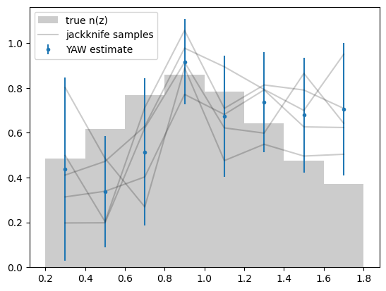
# true n(z)
zbins = handle_cross_corr.data.binning.edges
plt.hist(test_data["z"], zbins, density=True, color="0.8", label="true n(z)")

# fiducial n(z)
normalised = ncc.normalised()  # copy of data with n(z) is normalised to unity
ax = normalised.plot(label="YAW estimate")

# jackknife samples
normalised.samples.shape  # m jackknife-samples x n redshift slices
z = normalised.binning.mids
plt.plot(z, normalised.samples.T, color="k", alpha=0.2)
# create a dummy for the legend
plt.plot([], [], color="k", alpha=0.2, label="jackknife samples")
ax.legend()

DBG | normalising RedshiftData

<matplotlib.legend.Legend at 0x7f916834d060>

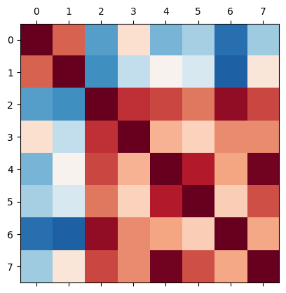
ncc.covariance.shape  # n x n redshift slices
ncc.plot_corr()

<Axes: >